They are tiny, invisible, and everywhere: viruses. Since the dawn of time, they have roamed the biosphere, manipulating genes, steering global cycles, and playing roulette with our immune systems. Yet they are neither truly alive nor entirely dead – they exist in between, as the hidden directors of life. Sometimes invisible guardians, sometimes treacherous invaders. And most of the time: completely unnoticed.
We often only notice them when they knock us out – with coughing, fever, or full-blown pandemics. Then, they suddenly become enemies, fearmongers, headlines. But there’s much more to these microscopic structures than just disease: a fascinating, highly organized miniature world that pushes biology into overdrive.
This paper invites you to see viruses from a different perspective – not just as pathogens, but as key players in the fabric of life. What makes them so successful? How do they reproduce with nothing more than a few genes? How do they influence ecosystems? And most importantly: do viruses even truly exist?
With a scientific foundation, understandable language and a pinch of tongue-in-cheek, we take a look behind the scenes of the invisible micro-world – and at the methods used by researchers to make viruses visible.
Curtain up for the invisible…
📑Inhaltsverzeichnis
1. Glimpse into the Invisible World
1.1. Guardians of Nature: Viruses as Regulators of Balance
1.2. Viruses as Drivers of Evolution
1.3. Do Viruses Really Exist?

2. Viral Mechanisms Illustrated by Influenza
2.1. How the Influenza Virus Travels
2.2. The Architecture of the Influenza Virus
2.3. The Infection Process of the Influenza Virus
2.4. The Adaptability of the Influenza Virus
2.5. Entry and Exit Routes of the Influenza Virus
2.6. Mostly Localized Mucosal Infection
2.7. Viral Strategy: Efficient Replication Without Rapid Cell Destruction
2.8. Destruction of the Host Cell
2.9. Self-Limiting Dangerous Viruses: Why They Rarely Cause Pandemics
2.10. Why Does the Virus Make Some People Sick and Others Not?

3. A Look at the Beginnings of Microbiology – How It All Started
3.1. Early Discoveries: The First Glimpses into the Invisible
3.2. The Birth of Modern Microbiology
3.3. The Step into the World of Viruses
3.4. Viruses and Koch’s Postulates

4. Modern Methods for the Discovery and Analysis of Viruses
4.1. Sample Collection
4.2. Sample Preparation
4.2. a) Filtration
4.2. b) Centrifugation
4.2. c) Precipitation
4.2. d) Chromatography
4.3. Cell Culture
4.4. Making Viruses Visible
4.4. a) Electron Microscopy
4.4. b) Crystallization
4.4. c) Cryo-Electron Microscopy
4.4. d) Cryo-Electron Tomography
4.4. e) Summary
4.5. The Genetic Fingerprint of Viruses
4.5.1. Nucleic Acid Extraction
4.5.2. Nucleic Acid Amplification
4.5.3. Sequencing
4.5.3. a) First Generation: Sanger Sequencing
4.5.3. b) Second Generation: Next-Generation Sequencing (NGS)
4.5.3. c) Third Generation: New Approaches in DNA Sequencing
4.5.3. d) Emerging Technologies: The Future of Sequencing
4.6. Bioinformatic Analysis

5. Do Viruses Really Exist?

6. Where Do Viruses Come From?
6.1. The Tree of Life
6.2. The Main Hypotheses on the Origin of Viruses
6.2.1. Hypotheses in a Cellular World
6.2.2. Hypotheses in the Pre-Cellular RNA World

7. Why Do Viruses Exist?
Epilogue: The Inconspicuous Ones

1. Glimpse into the Invisible World
Our visible world is only half the story – around us, on us, and within us exists an invisible universe full of microscopic players. Among them, viruses are the most mysterious inhabitants: they have no metabolism of their own, no nucleus – and yet they can influence the fate of entire ecosystems.
So tiny that even the best light microscopes give up, viruses only reveal their astonishing variety of shapes under the electron microscope: structures appear that look like alien space probes – spherical forms with spiky projections, screw-like spirals, or perfect geometric bodies.
Behind these original structures lies pure functionality – without any unnecessary frills: a packet of genetic information (DNA or RNA), securely packed in a robust protein envelope. Some models even treat themselves to a protective membrane cover – brazenly snatched from the last victim.
Simple yet effective: the recipe for viral success.

Let’s first zoom into this microworld to get a sense of the scale.
The mission of a virus: infect, reproduce, survive
Every virus has a clear mission: it must find a suitable host to reproduce and survive as a species. These hosts can be humans, animals, plants, or bacteria. There are even viruses that infect other viruses. Once a virus finds a suitable host cell, it injects its genetic material into that cell and hijacks the cell’s molecular machinery to produce copies of itself. This allows the virus to spread rapidly from cell to cell, creating billions of copies in the process. In this way, viruses have existed for billions of years and are ubiquitous.
The Life Cycle of a Virus: Dormant Phase vs. Attack Mode
A virus exists in two radically different states – almost like a double agent:
— The Extracellular Phase: The Virion —
Existence as a „nanospore“: an inactive but infectious particle.
Task: surviving outside host cells – on doorknobs, in droplets, in soil.
Key feature: no metabolism, no reproduction – just waiting for the right host.
Like a seed carried by the wind: inert, yet full of potential life.
— The Intracellular Phase: The Active Virus —
Brutal efficiency: A single virion can produce over 10,000 new viruses.
Mission Start: As soon as a suitable host cell is infected.
Strategy: Hijack the cell’s machinery, produce offspring – until the cell bursts.
Virion vs. Virus – Why the Distinction Matters
In science, every detail counts – even whether a virus is „dormant” or actively invading a cell.
- Virion: The infectious particle outside of cells – the traveling form.
- Virus: The generic term – includes both phases, inactive and active.
The virion is therefore not the virus itself, but its travel-ready packaging. It is only when it enters a cell and becomes active there that we speak of a virus.
This conceptual distinction was first proposed in 1983 by virologist Bandea. Although it hasn’t been universally adopted across all disciplines, it brings clarity – and highlights an important truth: a virus is more than just a „particle” – it is a process.
1.1. Guardians of Nature: Viruses as Regulators of Balance
The word „virus” instantly sets off alarm bells for most people: influenza, COVID, HIV, Ebola – disease, danger, pandemic. But this image represents only a tiny fraction of the truth. Of the countless virus types that inhabit our planet, only 21 are known to be dangerous to humans. The rest? Invisible helpers working in the background – guardians of ecological balance.
So no need to panic: most viruses couldn’t care less about us. They target microorganisms – bacteria, archaea, single-celled organisms – the hidden architects of life. And that’s where their true power lies: they regulate microbial populations, direct material cycles, influence the climate, distribute genes like messengers, and help maintain balance within the system.
There’s hardly a place on Earth where they can’t be found. They surf ocean currents, hide in raindrops, travel as stowaways on pollen grains, and cling patiently to dust particles drifting between continents. Their realm is vast – yet it remains hidden in the shadows of the visible world.
Mind-Boggling Numbers
With an estimated 100 million species, viruses are among the most abundant biological entities on Earth. Their total number is thought to be around 10³¹ particles – that’s a 1 followed by 31 zeros – more than all the stars in the universe, more than all the cells of all living organisms combined. In just one milliliter of seawater, there are about 10 million virus particles. Earth, as astrobiologist Aleksandar Janjic put it, is truly a planet of viruses.
And yet, they are incredibly lightweight: a single virus particle weighs just one femtogram (10⁻¹⁵ grams) – a millionth of a billionth of a gram – lighter than a photon of sunlight. Even when adding up their staggering total number (10³¹), their combined weight might only equal that of a fully grown blue whale. And still: without them, no balance, no cycles – no life as we know it.
But what makes them an integral part of the ecosystem?
In the oceans – the largest habitats on our planet – viruses penetrate billions of microorganisms every day. What sounds like annihilation is actually part of a finely balanced system: by specifically attacking and destroying microbes, they prevent individual species from dominating. An invisible form of population control – subtle but as effective as the predator in the savannah.
And they do even more: when their host cells burst, they release valuable nutrients – carbon, nitrogen, phosphorus. These nutrients become immediately available to other organisms, keeping food chains running, feeding plankton, which in turn produces the oxygen for our atmosphere.
At the same time, viruses act as evolution boosters. They transfer genes from one organism to another – a natural gene transfer that enables new traits, promotes diversity, and sparks innovation long before we even knew about genetic engineering.
And so it becomes clear: viruses are not mere carriers of disease. They are intricate cogs in the machinery of nature – unseen, rarely noticed, but indispensable.
A look into various habitats reveals their impact.
🌊 In the World’s Oceans
Population Control: Deep beneath the water’s surface, a microscopic battle of planetary scale rages on: bacteriophages – viruses that specifically infect bacteria – eliminate up to 40% of marine bacteria every day. By doing so, they prevent explosive algal blooms that could turn entire oceans into oxygen-deprived dead zones.
Without these „microbe hunters”, our planet would have long since sunk under a shroud of algae.
📖 Additional Sources:
Viral control of biomass and diversity of bacterioplankton in the deep sea
A sea of zombies! Viruses control the most abundant bacteria in the Ocean.
The smallest in the deepest: the enigmatic role of viruses in the deep biosphere
Gene Smuggling: In the blue depths of the oceans, Prochlorococcus – a tiny cyanobacterium – performs a mighty feat: it produces about 10% of the world’s oxygen. Yet even this microscopic hero is under the control of even smaller puppeteers: cyanophages – viruses perfectly specialized to infect it. These viruses insert their own photosynthesis genes and compel the infected cell to cooperate. The result: the bacterium remains „operational”, continuing to produce energy – now in service of its viral occupants. This parasitic partnership illustrates the so-called Black Queen Effect: by taking over certain functions, viruses allow microbes to lose those functions themselves and specialize in other tasks.
An involuntary division of labor, orchestrated by viruses.
Dive Deeper: An impressive glimpse into the mysterious world beneath the ocean’s surface is offered by a video from the Schmidt Ocean Institute. It showcases how researchers, using cutting-edge technology, follow the traces of microbial life – and in doing so, also track down viruses.
But viruses don’t just play this regulatory role in water – they are equally active in other ecosystems.
🟫 In the Soil
Even beneath our feet, viral activity is in full swing: viruses keep dominant soil bacteria in check, ensuring that no single microorganism gains the upper hand. This invisible regulation safeguards the delicate balance of the nutrient cycle – the foundation of all growth.
Like invisible gardeners, they comb through the micro-life of the Earth, weeding out excess and creating space for diversity.
🌳 In the Plant World
Trees and fields have secret allies: plant viruses. Around every root network unfolds a hidden web of control, defense, and opposition. Some plant viruses specifically target harmful bacteria that would otherwise sicken the plant. Others stimulate the plant’s own immune system – and when microbes die, viruses break down their remains into fertile compost. Some plants even go a step further: they actively recruit protective viruses that patrol the root zone like microscopic bodyguards.
Without these microscopic alliances, many forests would be far more vulnerable to fungal overgrowth – and our crops would be left defenseless against attacks from the soil.
🔗 Viruses as components of forest microbiome
🪱 In the Gut Flora of Humans and Animals
A silent power struggle also unfolds within our intestines – and we benefit from it. Specialized gut viruses (bacteriophages) specifically target harmful germs like E. coli, helping to maintain a stable bacterial balance. They transfer protective genes between microbes – like secret data packets that fine-tune immune responses. Some viruses even dampen overactive immune reactions, preventing inflammation in the process.
Without these nano-sheriffs, harmful bacteria would overrun the gut within days.
🔗 Over 100,000 Viruses Identified in the Gut Microbiome
☁️ In the Atmosphere
High above our heads, the largest gene transfer on Earth takes place – a single storm can disperse up to 500 million virions per square meter across entire continents, forming the ultimate bio-invasion route. Thanks to their extreme resilience, viruses survive where others fail – in UV-soaked altitudes, icy clouds, and dry air. They travel via dust, sea salt, or plant droplets across oceans and continents. Some even influence precipitation patterns by interacting with clouds.
This atmospheric gene exchange transforms local mutations into global evolution – as if nature had invented its own internet.
🔗 Deposition rates of viruses and bacteria above the atmospheric boundary layer
⚡️ In Extreme Habitats
Even in hot springs, salt lakes, or beneath the Earth’s crust, viruses thrive – regulating local microorganisms and boosting their genetic diversity. In these hostile environments, such regulation is an essential survival strategy.
🔗 Viruses in Extreme Environments, Current Overview, and Biotechnological Potential
The Greatest Paradox in Biology: From billions of microscopic acts of destruction arises global balance. So the next time you fear a virus, remember: with every breath, you carry billions of these tiny entities – and they, in turn, carry you. A pact of life – as old as evolution itself.
„We live in a balance, in a perfect equilibrium”, and viruses are a part of that, says Susana Lopez Charretón, a virologist at the National Autonomous University of Mexico. „I think we’d be done without viruses.” [Why the world needs viruses to function]
„If all viruses suddenly disappeared, the world would be a wonderful place for about a day and a half, and then we’d all die – that’s the bottom line”, says Tony Goldberg, an epidemiologist at the University of Wisconsin-Madison. „All the essential things they do in the world far outweigh the bad things.” [Why the world needs viruses to function]
1.2. Viruses as Drivers of Evolution
Long before dinosaurs roamed the earth, viruses were already up to mischief – shaping life as we know it today. Their tool: horizontal gene transfer, a biological copy-paste mechanism that enabled evolutionary quantum leaps.
For evolutionary biologist Patrick Forterre from the Pasteur Institute, viruses are the architects of life – without them, evolution might have taken a very different path.
(See also Spektrum der Wissenschaft: „The True Nature of Viruses”, ScienceDirect: „The origin of viruses and their possible roles in major evolutionary transitions” or „The two ages of the RNA world, and the transition to the DNA world: a story of viruses and cells”)
Genetic Sabotage with Lasting Effects
Viruses are masters of manipulation. When they infect a cell, they don’t just inject their own genetic material – sometimes their genes get integrated into the host’s genome and are passed down through generations. Supposed disruptors thus become creative gene architects.
A spectacular example: The placenta of mammals owes its existence to a virus. A viral envelope protein – originally designed to suppress immune responses – was incorporated into the gene pool and helped develop the barrier between mother and embryo. Without this „foreign” gene: no womb, no mammal.
But it goes even further: about 8% of the human genome comes from ancient retroviruses that once embedded themselves into our DNA – silent witnesses of ancient infections that may still influence us today. Even our brain might carry viral traces – for example, genes crucial for the development of the cortex.
Aren’t we all a bit of a virus?
CRISPR, celebrated today as a revolutionary gene-editing tool, traces back to an ancient bacterial defense system – a genetic archive of past viral attacks from which bacteria learn to defend themselves against new enemies.
Some scientists even ask: Could viruses have played a role in the origin of life itself? Certain hypotheses suggest that virus-like particles may have been the first molecules capable of storing and transmitting genetic information – a fundamental prerequisite for life.
The irony of fate: We fear viruses as bringers of death – yet without them, we might never have come into existence.
1.3. Do Viruses Really Exist?
Despite their immense importance, there are always doubts about the existence of viruses. How can we be sure that they are real? This question cannot be answered by simple observation – viruses elude our naked eye and only reveal themselves through indirect traces and specialized detection methods.
To get to the bottom of this question, we first need to understand how viruses act: What mechanisms do they use to replicate? How do they interact with their hosts? And above all, what scientific methods are available to visualize and detect them?
The search for these answers leads us into a fascinating world of advanced technologies and decades of research. In the chapters to come, we will explore step by step how scientists detect viruses – bringing us closer to answering the essential question: Do viruses really exist?

2. Viral Mechanisms Illustrated by Influenza
Let’s begin by taking a closer look at how viruses „hijack” their host cells and exploit them for reproduction. A prime example of this is the influenza virus – not only because it is one of the most thoroughly studied viruses, but also because it vividly demonstrates how viruses manipulate cells and spread. The mechanisms it employs offer us an ideal insight into the mysterious world of viruses and their complex interactions with their hosts.
2.1. How the Influenza Virus Travels
2.2. The Architecture of the Influenza Virus
2.3. The Infection Process of the Influenza Virus
2.4. The Adaptability of the Influenza Virus
2.5. Entry and Exit Routes of the Influenza Virus
2.6. Mostly Localized Mucosal Infection
2.7. Viral Strategy: Efficient Replication Without Rapid Cell Destruction
2.8. Destruction of the Host Cell
2.9. Self-Limiting Dangerous Viruses: Why They Rarely Cause Pandemics
2.10. Why Does the Virus Make Some People Sick and Others Not?
💡Note: The following chapters build upon basic knowledge of cells, the difference between DNA and RNA, proteins, and cellular processes such as protein biosynthesis. If these topics are still new to you, it may be helpful to take a look at Chapters 2, 3, and 4 of the treatise „The Wonderful World of Life” or similar introductory texts.
Chapter 2: The Cell – The Fundamental Building Block
Chapter 3: Proteins – The Building Blocks of Life
Chapter 4: From Code to Protein – Cellular Mechanisms
2.1. How the Influenza Virus Travels
The influenza virus is constantly on the move – an invisible jet-setter with astonishing transmission routes: sometimes it travels first class via a sneeze cloud, other times it hitchhikes over door handles.
Droplet flight – first class through the air
One sneeze is enough: up to 40,000 virus-laden droplets shoot through the air – like a mini missile strike on the surroundings (range: up to 2 meters!).
Smear attack – the secret handshake
Door handle, elevator button, keyboard – the virus chills on surfaces, sometimes for hours. One touch, one swipe of the face – and it has already gained access via a hand-to-face trick.

Mission: Respiratory Tract – Viral Invasion
Once inside the respiratory tract, the virus launches its assault on epithelial cells:
Preferred target: Mucosal cells in the nose, throat, and bronchi.
Why? There are plenty of favourite receptors here – perfect docking sites.
Result: Within hours, it hijacks the cell’s machinery and begins producing new viruses.
From the outside, it looks like a speck of dust with bad intentions – but upon closer inspection, the influenza virus reveals itself as a highly complex nanomachine. To understand how it hijacks cells and constantly mutates, it’s worth taking a closer look inside.
2.2. The Architecture of the Influenza Virus
The influenza virus is the reason we find ourselves bedridden with fever, cursing „the flu”. Of the three strains (A, B, and C), Type A is the most dangerous globetrotter: as shape-shifting as an actor and as unpredictable as April weather. Types B and C, on the other hand, are more „down-to-earth” – less variable and generally less dangerous. Yet all of them share the same ingenious structural blueprint (see illustration below).
The virus particle – a mere 80 to 120 nanometers in size – is a master of survival, resembling a tiny, spherical nano-submarine (sometimes oval-shaped). Inside: its viral genetic material made of RNA – but with a special trick!
While we often think of RNA or DNA as a single, unbroken strand, viruses have different DNA and RNA structures. Some have a single continuous molecule, others carry their genetic material divided into several RNA segments.
The Command Center: Genome in 8 Segments
The influenza virus is based on a modular design: it uses 8 separate RNA segments – like a construction kit whose parts can always be recombined – perfect for surprises!
These RNA segments vary in length – from compact mini-modules to XXL construction manuals – and yet they are perfectly harmonised. To prevent them from getting lost like loose pages in the wind, each segment is carefully packaged: every strand is wrapped in a sheath of nucleoproteins (NP), like precious scrolls in protective foil. But the NP envelope is more than just protection: it assists the viral machinery to precisely read, copy and pass on the genetic information.
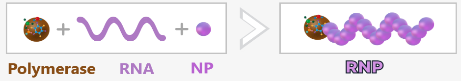
The toolbelt: Polymerase complexes
In addition, the virus brings its own 3D printers – the RNA polymerases (composed of the subunits PB1, PB2, and PA). These are firmly attached to the RNA segments, like craftsmen carrying their tools on a belt.

The RNP Complex – the Heart of the Virus
Each RNA segment + nucleoproteins (NP) + polymerase forms a ribonucleoprotein complex (RNP) – a perfectly organized unit: the virus’s command center. All eight – neatly packed and ready for action – like a portable toolbox for taking over the cell.
The Lipid Envelope – the Stolen Cloak of Invisibility
The virus steals its outer layer directly from the host cell: a lipid bilayer – identical to the cell membrane, making it the perfect disguise! Just beneath it lies the matrix protein M1 – the molecular scaffolder that holds everything together. It connects the outer envelope with the inner complex and ensures the virus keeps its shape – like a support frame beneath the cloak.
The Spikes: Key & Scissors
Embedded in the viral envelope are crucial surface proteins that protrude like tiny spikes or grasping arms. These are called „spikes”. The influenza virus has two especially important spikes that help it infect cells: Hemagglutinin (HA) and Neuraminidase (NA).
🔑 HA – The Door Opener: Acts as a key to dock onto the host cell.
→ 18 known variants (H1–H18)
✂️ NA – The Escape Helper: Breaks the connection to the host cell so the virus can move on.
→ 11 variants (N1–N11)
Virus Types: A Numbers Game
The combination of HA and NA determines the strain:
- H1N1 (swine flu)
- H5N1 (avian flu)
- H3N2 (seasonal flu)
Like car license plates: HA/NA codes reveal which „model” is on the move – just without road safety inspection!
2.3. The Infection Process of the Influenza Virus
a) Attachment of the virus to the host cell (Adsorption)
b) Entry into the cell (Endocytosis)
c) Release of the viral genetic material (Uncoating)
d) Viral replication – The molecular factory
e) Assembly of new virus particles
f) Budding and release of new viruses
a) Attachment of the Virus to the Host Cell (Adsorption)
The surface of the respiratory tract is lined with a dense epithelium of mucosal cells. These cells carry sialic acid residues on their surface – sugar molecules that play a central role in cell communication and immunological self-recognition (see chapter „SELF Markers: Sialic Acids” in „The Wonderful World of Life”).
The influenza virus hijacks this mechanism: its surface protein hemagglutinin (HA) specifically binds to the sialic acid of the host cell – a classic lock-and-key interaction that initiates the virus’s entry.

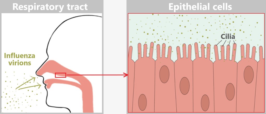
Before the influenza virus can infect a cell, it must first attach to the host cell – a crucial step in the infection process. However, the epithelial cells of the respiratory tract are not defenseless: their motile cilia (tiny hair-like structures) transport foreign particles such as dust, bacteria, or viruses away before they can reach the cell surface.
The illustration shows the relative sizes at the cell surface. The cilia are 5–10 micrometers long, while the mucus layer has a thickness of 10–100 micrometers. At just 80–120 nanometers, the virus particle is tiny. It must quickly reach a cell before the cilia carry it away.
Between the cilia, there are exposed areas of the cell surface where the virus can make direct contact. The sialic acid residues (1 nanometer) on the host cell membrane serve as docking sites for the HA protein (13 nanometers) of the virus, which is large enough to reach these structures. This allows the virus to penetrate the mucus layer and bind to the host cell.
b) Entry into the Cell (Endocytosis)
The influenza virus is a master of disguise: by binding its hemagglutinin to sialic acid residues, it mimics a harmless nutrient molecule. The host cell falls for the trick and initiates its standard uptake mechanism – endocytosis.
What follows is a molecular spectacle:
The cell membrane folds around the attached virus – triggered by signaling molecules normally responsible for nutrient uptake. Like a closing trap, an indentation forms that fully engulfs the virus. With a final „snap” of the membrane, an endosome is formed – a transport vesicle that now innocently shuttles the intruder into the cell’s interior.
What the cell registers as harmless transport turns out to be a Trojan horse.

The virus is now inside the cell – still enclosed within the endosome – but ready to unfold its innermost potential.
c) Release of the Viral Genetic Material (Uncoating)
The early endosome matures into a late endosome – a site where the cell typically degrades unwanted intruders. Proton pumps lower the pH by transporting protons (H⁺ ions) into the interior, creating an acidic environment intended to activate digestive enzymes.
The acidic trick
But the influenza virus has a brilliant counterplan: the acidic environment triggers a dramatic transformation of the viral hemagglutinin (HA). The protein splits – its binding domain HA1 is cleaved off, and the fusion domain HA2 is exposed.
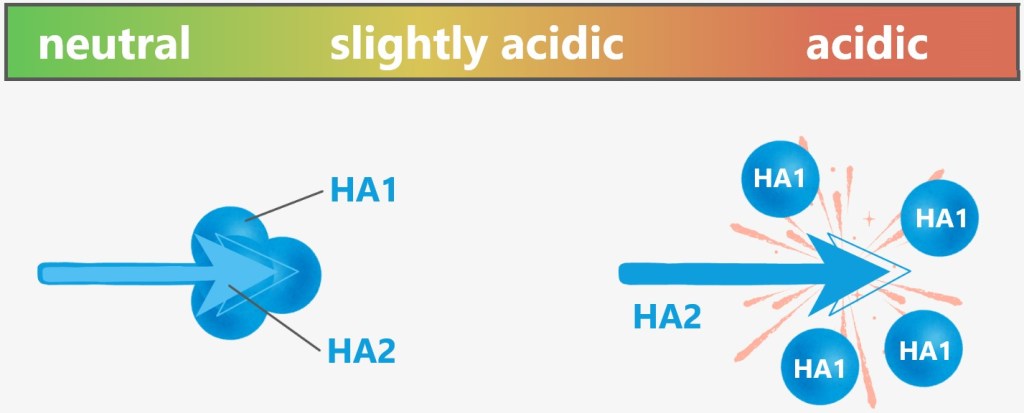
This fusion domain, HA2, is hydrophobic – it avoids water – and rams itself like a grappling hook into the endosomal membrane (see illustration below).
At the same time, the M2 protein – a viral ion channel – acts as a secret accomplice and opens the floodgates: protons flow into the virus interior, loosening the packaging of its genetic material.

Now, HA2 pulls the viral membrane and the endosomal membrane together with relentless force. The two lipid membranes fuse – a process known as membrane fusion. This occurs because the lipid molecules in the membranes are flexible and can rearrange themselves to form a continuous bilayer.

This fusion creates a pore – the gateway to freedom for the viral genome. With one final, elegant push, the viral RNA slides into the cytoplasm. The uncoating process is complete.
The cell has no idea that it has just released the blueprint for its subjugation.
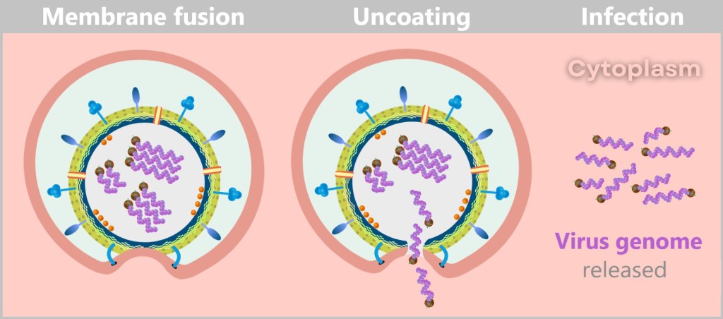
Through membrane fusion and uncoating, the viral envelope is dissolved, releasing the genome and initiating the infection.
Why is the virus not degraded?
The virus is not degraded by the cell’s digestive enzymes because the release process happens quickly – before the degradation mechanism (activation of digestive enzymes) can take effect. The virus exploits the drop in pH and the changes within the endosome to rapidly escape by triggering membrane fusion, releasing its genome directly into the cell’s cytoplasm. This „escape” from the endosome is faster than the cellular breakdown process, which is why the virus is not decomposed.
d) Viral Replication – The Molecular Factory
The viral RNA does not arrive unprotected – it travels in high-tech armor: wrapped in protective nucleoproteins (NP) and equipped with viral polymerase, each of the eight RNA segments forms a highly organized ribonucleoprotein complex (RNP). These molecular command units are perfectly equipped for their mission:
- The nucleoproteins act like armor – shielding the RNA from cellular defense systems.
- The polymerase is the Swiss army knife of the virus – a tool for copying (replication) and translating (transcription) in one.
As soon as the ribonucleoprotein complexes (RNPs) are released in the cytoplasm, the systematic takeover of the cellular production lines begins – the virus factory goes into operation. The genome takes on two central tasks: On the one hand, it serves as a blueprint for the production of viral proteins (Protein synthesis), on the other hand, it is itself replicated (Genome replication) – so that each new virus particle is given its own copy of the genetic material along the way.

Protein synthesis: The viral genome serves as a template for the synthesis of the proteins needed to assemble new virus particles.
Genome replication: At the same time, the viral RNA is replicated to provide the genetic information for new viruses.
While most RNA viruses remain in the cytoplasm, influenza has a clever trick up its sleeve: it hijacks the cell nucleus. Why? Because there, it finds optimal conditions for replicating its RNA.
The journey there, however, is anything but straightforward. The RNPs manipulate the cellular transport system by presenting fake import signals – molecular entry passes that grant them access to the nucleus. Cellular importins, normally responsible for transporting the cell’s own proteins, thus become unsuspecting smugglers. In a feat of biological deception, the viral RNPs are escorted straight into the cell’s control center.

In the cell nucleus, the RNPs finally unfold their full potential. The viral polymerase begins its double role:
- Copying the viral RNA (replication) → blueprint for new viruses
- Producing viral mRNA (transcription) → building instructions for protein synthesis
As this process is particularly sophisticated, each step is described in detail below.
1️⃣ Activation of the RNA polymerase – Here we go
The viral polymerase needs a molecular ignition spark to become active. And it finds this in the cell nucleus: a biochemical special zone that differs significantly from the cytoplasm. High concentrations of nucleotides, ions and nucleus-specific factors send a clear signal: „This is the place to start!” Only in this environment does the polymerase come to life. Without this molecular wake-up call, it remains in a dormant state – camouflaged as a harmless cellular component.
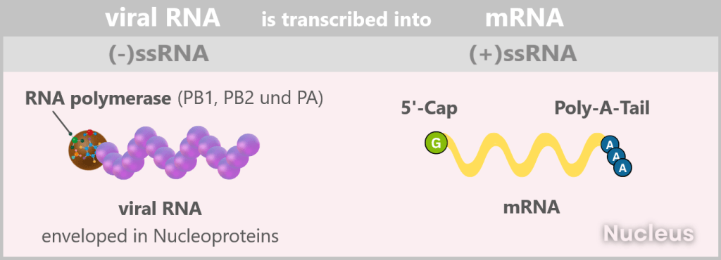
2️⃣ Initial situation: (-)ssRNA – A Genome in Mirror Writing
The genome of the influenza virus is a master of disguise. Instead of presenting itself as a readable blueprint, it appears more like a riddle in mirror writing: eight separate RNA segments, negatively polarized, lacking all the usual hallmarks of a cellular message. No sender, no letterhead, no stamp. To the cell, it’s not a message – it’s biological noise.
In scientific terms:
The viral genome consists of eight segmented single-stranded RNA (ssRNA) with negative polarity: (-)ssRNA. „Negative” means that this RNA is the complementary template to the mRNA (i.e. mirror-inverted) and therefore not directly readable.
In addition, it lacks two crucial identifying features: the 5′ cap (a kind of molecular start button) and the 3′ poly-A tail, which protect and identify a normal mRNA.
Why so complicated?
Because it’s brilliant.
With this molecular masquerade, the virus achieves two things:
Staying invisible: The (-)ssRNA is not immediately recognized as a threat by the cell’s immune system. If the viral genome were already in the form of mRNA, the cell’s alarm systems would be triggered right away.
Full control over production: The virus doesn’t beg for help from the host’s enzymes. Because only the virus’s own RNA polymerase can convert the (-)ssRNA into readable mRNA, the virus can precisely control:
➤ When mRNA is produced.
➤ How much of it is produced.
➤ Which segments are prioritized.
In short: What looks like a cryptic puzzle is actually a highly precise control mechanism – a blueprint that only reveals itself when the viral machinery is ready – and the immune system is still asleep.
3️⃣ From (-)ssRNA to (+)ssRNA (the mRNA)
The viral polymerase is ready to transcribe the (-)ssRNA into readable mRNA – but the start button is missing. Without the 5′-cap, the machinery remains silent.
The solution? Theft at nano level.
This ingenious trick is called cap-snatching.
The Coup in Detail
The polymerase subunit PB2 prowls through the cellular mRNAs like a cunning thief searching for the most valuable jewel. Its target: the 5′ cap, the universal „seal” for cellular protein factories. Its accomplice, PB1 – the „molecular scissors” – cuts off the cap along with 10–15 nucleotides – a perfect primer for viral transcription. The stolen cap is attached to the viral RNA. The cell believes it has a legitimate mRNA and starts producing viral proteins. Meanwhile, the capped host mRNA is degraded – causing the collapse of the cell’s protein production.
At the same time, the viral mRNA receives a poly-A tail at its 3′ end, which stabilizes and protects it.
Why this trick is so brilliant
✅ Energy-saving: The virus uses existing resources – no effort needed to synthesize its own cap.
✅ Sabotage: The degradation of cellular mRNAs cripples the host’s defense.
✅ Camouflage: The stolen cap disguises viral mRNA as a „harmless” cellular message.
The Consequences of the Heist
- The cell loses its own blueprints – and now produces viral proteins at full speed.
- The virus gains twice: rapid replication and weakening of its adversary.
This process is a classic in virology – a prime example of how viruses turn their host cells into puppets.
In the end, numerous „naked” +ssRNA strands are produced in the cell nucleus, which are used directly as mRNA for translation, i.e. for viral protein production and genome replication.
4️⃣ The virus production is running hot
The freshly capped viral mRNAs exit the nucleus – equipped with a stolen signature and a poly-A tail. In the cytoplasm, ribosomes are waiting, unsuspectingly executing the enemy’s blueprints.
The prey: an entire protein factory
The ribosomes churn out viral proteins on an assembly line – including:
Haemagglutinin (HA): The key to cell entry – the indispensable door opener.
Neuraminidase (NA): The liberator of new viruses – the sharp molecular scissors.
Matrix protein (M1): The stable envelope for the virus interior – the scaffold builder.
Ion channel protein (M2): The pH guardian – regulates the acidic environment in the virus.
RNA Polymerase (RNAP): The copying machine – a viral printing press.
Nucleoprotein (NP): The bodyguards – package and protect the RNA segments.
Nuclear Export Protein (NEP): The dispatcher – handles the export of viral RNPs from the nucleus.
These freshly produced proteins are ready for the final act: the assembly of new virus particles.
5️⃣ Return to the Nucleus
After being produced in the cytoplasm, most viral proteins make their way back to the nucleus – the command center of viral replication. The only exceptions are the surface stars: hemagglutinin (HA), neuraminidase (NA), and the ion channel protein M2, which operate directly at the cell membrane.
The remaining viral actors return to headquarters to pick up new orders and prepare for the final mission.
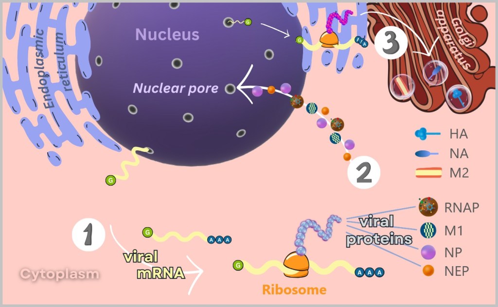
1) At free ribosomes in the cytoplasm, the mRNA is translated into viral proteins such as RNA polymerase, matrix proteins (M1), nucleoproteins (NP), and nuclear export proteins (NEP).
2) These proteins then migrate back into the nucleus to participate in the replication and packaging of the viral genome.
3) The surface proteins (HA and NA) and the ion channel protein (M2) are synthesised at the membrane-bound ribosomes of the endoplasmic reticulum (ER). After their production, these proteins are transported to the Golgi apparatus, where they are further modified and prepared for incorporation into the viral envelope.
6️⃣ The Genome Copy Factory: (+)ssRNA → new (-)ssRNA
While viral proteins are being mass-produced in the cytoplasm, a covert operation „Genome Replication” unfolds in the nucleus:
Newly formed RNA polymerases grab the freshly synthesized (+)ssRNA strands and transcribe them back into viral mirror-image RNA – producing new (−)ssRNA strands. The polymerase remains bound as an integrated printing press for future rounds.
Nothing is left to chance: Even as the genetic code is being reverse-transcribed, nucleoproteins (NP) coat the emerging (−)ssRNA – it doesn’t spend even a second „naked” – eliminating any risk of cellular surveillance. The freshly copied RNA segments are immediately packaged and sealed: Together with the polymerase, they form complete ribonucleoprotein complexes (RNPs) – fully equipped genome modules, ready for the next generation of virus.
Once the eight segments are packaged, the viral logistics team takes over: NEP (nuclear export protein) and M1 (matrix protein) tag the RNPs for export. They escort them through the nuclear pores – the cell’s heavily guarded gateways – directly into the cytoplasm. Mission: assembly hall.

1) The viral RNA polymerase uses the (-)ssRNA as a template to synthesize a complementary (+)ssRNA.
2) This (+)ssRNA then serves as a template for the renewed synthesis of viral (-)ssRNA – the actual genetic material for new virus particles.
3) Already during synthesis, the new (-)ssRNA is coated with nucleoproteins (NP) and packaged with polymerase, M1, and NEP into the so-called RNP complex – stable and ready for export.
4) The completed RNP complexes exit the nucleus through the nuclear pores and migrate into the cytoplasm – where the assembly of new viruses soon begins.
Like a clandestine printing shop in the back room: The polymerase continuously produces copies, the NP proteins immediately package them, and smugglers (NEP/M1) discreetly sneak them out.
While the cell unsuspectingly burns through its resources, the real showdown is still ahead…
e) Assembly of New Virus Particles
Once all the components have been produced, the coordinated final assembly begins in the cytoplasm – a process as precise as the construction of a space probe: every part has to fit perfectly, otherwise nothing will lift off.
The surface proteins HA & NA travel through the Golgi apparatus – the cell’s „packaging department” – to the cell membrane (see lower left illustration). There, they anchor themselves in the lipid bilayer like door handles and rescue scissors protruding from the envelope of a future virus particle.
The ribonucleoprotein complexes (RNPs) also set out on their journey, already in tow of the matrix proteins M1, which act as logistics managers. Their task: to reliably navigate the valuable cargo to the membrane regions equipped with HA and NA (see lower right illustration).
At the cell membrane, the viral puzzle comes together piece by piece: The RNPs arrange themselves beneath the membrane studded with HA and NA. The matrix proteins assist in bringing the RNPs into contact with specific regions of the cell membrane.
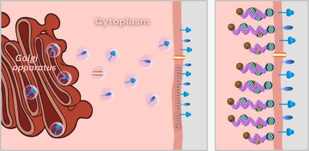
Left: Incorporation of viral surface proteins (HA and NA) and the ion channel protein (M2) into the cell membrane.
Right: Transport of ribonucleoprotein complexes (RNPs) to the cell membrane and their attachment to the forming viral envelope.
And now – drumroll please – everything is set for the grand breakout!
f) Budding and Release of New Viruses
A protrusion forms on the cell membrane – like a soap bubble with a deadly cargo. But what looks so playful is actually precise choreography:
➤ Viral proteins push outward, causing the lipid bilayer to curve into a perfectly shaped „virus package”.
➤ Matrix proteins (M1) stretch the membrane like a trampoline – stable, but flexible enough for the jump.
➤ The host lipids close to form a camouflaged envelope – the virus packages itself.
But it is not yet free. Sialic acid tethers lurk on the cell surface – normally HA’s favourite anchorage. Without resistance, the virus would stick like chewing gum under the sole of a shoe.
Neuraminidase (NA) steps in: the molecular scissors slice through the sialic acid residues on the cell surface. No sticking, no turning back – a clear path to the next cell.
Like a jailbreak with style: M1 loosens the bars, NA cuts the alarm wires – and they’re gone! Final countdown for the virus crew! All systems go – HA/NA check, RNPs check, lipid armor check. Launch sequence initiated in 3…2…1… Budding!

Left: Budding of the virus at the cell membrane. Right: Release of the newly formed virus particle.
The following video provides a clear and accessible summary of the replication cycle of the influenza virus.
After a host cell is infected by a single influenza virus, hundreds to thousands of new virus particles are typically produced. The exact number can vary and depends on several factors, such as the virus strain, the type of host cell, and the cellular conditions.
Simplified and Realistic Representation of the Virus Structure
In the initial illustrations of this text, the structure of the influenza virus was simplified for better clarity (see bottom left image). In these illustrations, the matrix protein is shown as a spherical, mesh-like ring structure surrounding the viral genome. This simplified representation is intended to make the complex processes of viral replication easier to understand.
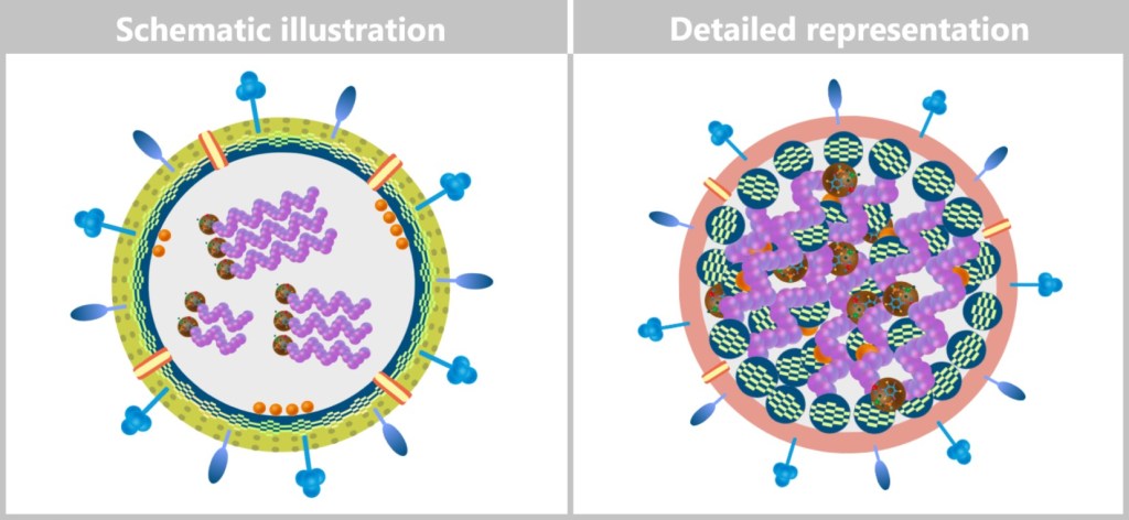
Left: Schematic illustration to clarify the structure of the virus.
Right: More detailed schematic representation of the virion structure.
In the following illustrations, however, the structure of the new virions is depicted in a way that more closely reflects biological reality. The matrix proteins are not shown as a continuous ring, but are located in individual units that both bind to the inner lipid layer and are loosely linked to the ribonucleoprotein complexes (RNPs). In addition, the colouring of the lipid layer reflects the origin from the cell membrane of the host cell (see upper right figure).
The RNPs representing the viral genome are arranged inside as a loose bundle – not strictly parallel, but flexibly organized with ends oriented in different directions. The matrix proteins (M1) hold this bundle together and connect it to the lipid layer, giving the virion its shape and stability.
2.4. The Adaptability of the Influenza Virus
Viruses – especially RNA viruses like the influenza virus – mutate extraordinarily fast. The reason lies in their error-prone replication machinery: the viral RNA polymerase lacks a mechanism to correct copying errors, unlike DNA replication in human cells. As a result, random mutations – small changes in the virus’s genetic material – occur with each replication cycle.
Within an infected person, this process produces a multitude of slightly different virus particles. Most mutations are neutral, meaning they neither affect the virus’s function nor its ability to replicate. However, some mutations are disadvantageous, causing the virus to replicate less efficiently or lose infectivity entirely – these variants quickly disappear through natural selection.
But some mutations give the virus a survival advantage, especially when they affect the surface proteins hemagglutinin (HA) and neuraminidase (NA). These proteins are key targets of the immune system: the body produces antibodies that specifically bind to them and neutralize the virus. However, if the structure of HA or NA changes due to mutations, the antibodies recognize the virus less effectively. The virus essentially becomes „invisible” to the immune defense and can continue to replicate and spread.
This constant adaptation explains why influenza viruses cause new waves of infection every year and why it is challenging to develop long-lasting vaccines against the flu.
The influenza virus does not exist as a fixed genetic entity but rather as a so-called mutant cloud (quasispecies) – a dynamic population of viral variants arising through continuous mutations. This genetic diversity is key to its survival: natural selection ensures that the variants most successful under the given conditions prevail. This high adaptability of the influenza virus vividly demonstrates how evolution occurs in real time.

The influenza virus must constantly change through mutations to continue existing as the flu virus. The high mutation rate leads to a multitude of slightly different viral particles within an infected person.
2.5. Entry and Exit Routes of the Influenza Virus
Influenza viruses use the mucosal surfaces of the respiratory tract as their entry point, since mucous membranes form the boundary between the external environment and the inside of our body. Many viruses initiate infection by interacting with the epithelial cells of these mucous membranes in order to spread efficiently within their host. [Virus Infection of Epithelial Cells]
As shown in the illustration below, the influenza virus enters the respiratory tract via the air – reaching the nose, throat, and lungs – and binds to the apical side (upper surface) of the epithelial cells, which faces the external environment. This apical side is covered with fine, hair-like structures called cilia, which help transport mucus and foreign particles. The opposite, basolateral side of the cell faces the underlying tissue and is connected to the basement membrane, anchoring it to the connective tissue.

The release of newly formed influenza viruses also occurs specifically at the apical side. This arrangement allows the viruses to spread into the surrounding environment – such as through droplets expelled by coughing or sneezing – thereby easily infecting new hosts. This apical release represents an evolutionary advantage, as it significantly enhances transmission efficiency.
2.6. Mostly Localized Mucosal Infection
Influenza viruses are specialized for infections of mucosal surfaces. As a result, their infection typically remains localized to the epithelial cells of the respiratory tract, meaning it is confined to a mucosal infection. The virus spreads from cell to cell along the apical side of the epithelial layer, without penetrating deeper tissue layers. Even when the infection progresses from the upper respiratory tract down to the lungs, it remains limited to the mucosal surface.
The basolateral side of epithelial cells usually remains untouched, as it plays no role in viral transmission. If the virus were to exit the host cell from the basolateral side, it could spread into the surrounding tissue and ultimately enter the blood or lymphatic system, potentially leading to a systemic infection. However, for influenza viruses, this would be disadvantageous: they would face stronger immune defenses and their transmission via the respiratory tract would become more difficult.
In rare cases – particularly in severely immunocompromised individuals – the virus can break through the epithelial barrier and invade the underlying tissue as well as blood or lymphatic vessels, leading to a systemic infection.
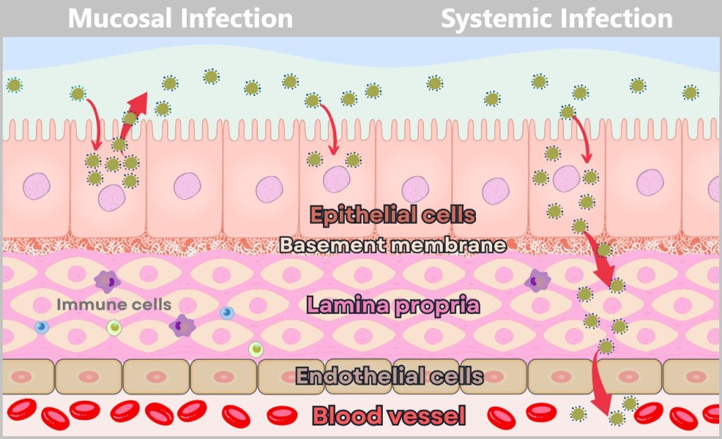
The mucosa consists of several layers: Epithelial cells form the outer protective layer, the basement membrane acts as a thin barrier, the lamina propria supports with connective tissue and immune cells, endothelial cells form the walls of blood vessels, and the blood vessel leads into the interior of the body.
Left – Mucosal infection (limited to the mucosal surface): The virus infects epithelial cells exclusively via the apical side. It remains within the mucosa, spreading from cell to cell along the apical surface. The basement membrane and underlying tissues such as the lamina propria remain intact. A mucosal infection is locally restricted and favors transmission via mucosal surfaces, such as the respiratory tract.
Right – Systemic infection (spread through the bloodstream): The virus enters the epithelial cells on the apical side but exits them via the basolateral side. It breaches the basement membrane and moves through the lamina propria, either by migrating or infecting cells there. Eventually, it reaches a blood vessel by passing through gaps between endothelial cells or by directly infecting the endothelial cells. Entry of the virus into the bloodstream marks the transition to a systemic infection. A systemic infection is critical because the virus can then spread throughout the body via the blood, potentially damaging vital organs such as the lungs, heart, or brain.
2.7. Viral Strategy: Efficient Replication Without Rapid Cell Destruction
Some viruses – including influenza viruses – are surprisingly economical: instead of destroying their host cell immediately, they exploit its resources as efficiently as possible. Why burn down the apartment if you can live rent-free for months? As long as the cell remains intact, it provides everything the virus needs for replication: energy, enzymes, building blocks. The immune system also notices something’s wrong only later – because if nothing’s on fire, no alarm is triggered. This strategy prolongs the life of the infected cell, delays the immune response, and maximizes the production of new viruses.
Virus wisdom: The best parasites stay under the radar!
2.8. Destruction of the Host Cell
What starts as cunning protection ends in molecular burnout: the infected cell ultimately suffers cell death. This occurs when the cell is either overloaded and structurally damaged by the massive production of viruses, triggered to enter programmed cell death (apoptosis) by cellular defense mechanisms, or deliberately eliminated by the immune system. These characteristic changes in the host cell caused by the virus are referred to as cytopathic effects (CPE). This entire process can take place within as little as 24 hours after infection.
To better understand cell death caused by influenza viruses, let’s examine the three mechanisms by which the host cell is ultimately destroyed.
a) Overload and structural damage
b) Apoptosis: programmed cell death to combat the virus
c) Immune response: Destruction by the immune system
a) Overload and structural damage
The virus takes over the cellular processes to produce its own components. With each new generation of viral proteins and RNA, the cell’s energy and resource capacity become increasingly depleted. Since the cell practically works only for viral replication, its own vital functions come to a halt. The cell becomes a squeezed lemon – ribosomes run hot, mitochondria collapse.

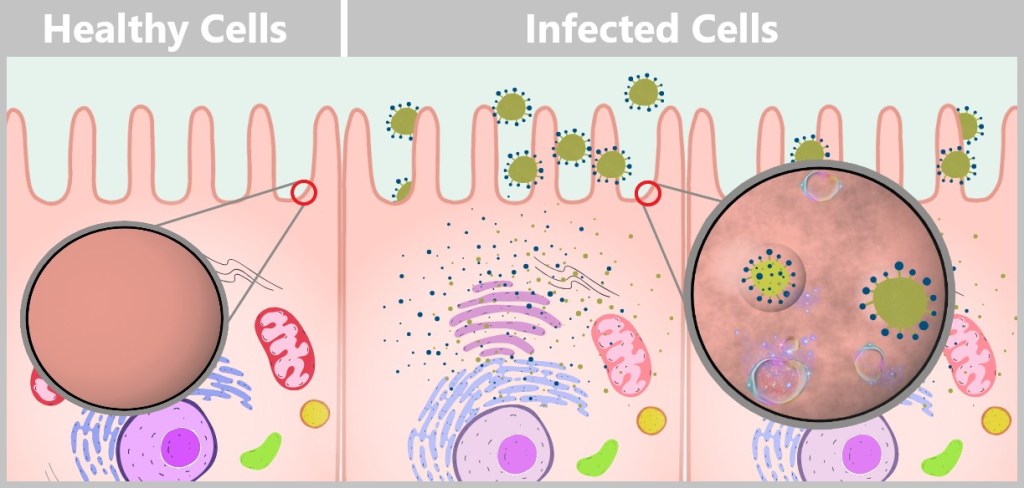
Left: Healthy cell with fully functional cellular machinery. The cell’s own mRNA (orange) is read by ribosomes to produce proteins necessary for cellular functions. The cell displays vibrant staining, indicating full resource capacity and energy availability.
Right: Virus-infected cell, heavily burdened by the production of viral components. The viral mRNA (yellow) increasingly displaces the cell’s own mRNA, and the ribosomes predominantly read viral instructions for virus replication. The pale staining of the organelles symbolizes the depletion of energy reserves and the overload of the cell.
During budding at the cell membrane – when new virus particles exit the cell – the membrane is repeatedly pierced and deformed. This process ultimately leads to the loss of membrane integrity, causing the cell to lose its stability and protective functions. The cell eventually dies due to relentless resource depletion and structural breakdown resulting from virus release.
During budding, the cell membrane forms small protrusions from which new viruses are released. Each budding event removes tiny portions of the membrane’s lipid bilayer, as the newly forming viruses use the host cell’s membrane material for their envelope. After repeated viral release, the membrane becomes significantly thinned and structurally weakened, often showing deformations and irregularities. The constant stress from budding makes the membrane more porous and vulnerable. The cell increasingly loses its ability to regulate its internal environment and can hardly maintain its selective permeability for ions and molecules. As membrane damage continues, its structural stability deteriorates. Eventually, the membrane may become so compromised that it ruptures or disintegrates, ultimately leading to cell death.
b) Apoptosis: programmed cell death to combat the virus
When a cell realizes it has been hijacked, it sometimes pulls the emergency brake – sacrificing itself for the greater good: it commits suicide to stop the virus from spreading. The plan: take the enemy to the grave. Instead of dying with a bang, the cell undergoes a controlled breakdown into small fragments called apoptotic bodies, which are then cleared away by immune cells.
This process follows a precise sequence: the DNA is fragmented, the cell membrane forms characteristic bubble-like protrusions (known as blebbing), and internal structures are neatly dismantled and recycled. The cell dies quietly – and in doing so, protects the organism.
This mechanism proves – cells have more honor than some governments!

Healthy Cell: On the left, an intact cell is shown with an undamaged cell membrane and nucleus. The nucleus contains complete DNA strands, and the cell shows no signs of stress or damage.
Infected cell – initiation of apoptosis: In the middle section, the cell begins to show visible changes. The cell membrane forms bubble-like protrusions (blebbing), and the nucleus starts to shrink. Within the nucleus, fragmented DNA becomes visible, resulting from apoptotic processes. This phase marks the transition from a functioning cell to its controlled disintegration.
Apoptotic Bodies and Degradation: On the right, the cell breaks apart into several small fragments known as apoptotic bodies. In the background, an immune cell (macrophage) is shown engulfing and degrading these fragments. This process prevents the release of viral components and protects the surrounding tissue from further infection.
c) Immune response: Destruction by the immune system
Once the immune system detects a virus-infected cell, it sounds the alarm – and that spells trouble for the virus! Specialized fighters like natural killer (NK) cells and cytotoxic T cells leap into action. They identify infected cells by viral protein signals that wave like warning flags on the cell surface. With deadly precision, they release toxic molecules, destroy the infected cell, and effectively slow down viral replication!
Anyone curious to learn more about this fascinating defence battle can find detailed information in „The Wonderful World of Life”, especially in Chapter 5.3 d) „Natural Killer Cells” and Chapter 5.5.7 b) „Cytotoxic T Cells”.
NK cells and cytotoxic T cells form an unbeatable team – they hunt down and eliminate viral threats, keeping the infection under control.
Regeneration of Epithelial Cells
As previously mentioned, the influenza virus primarily infects the epithelial cells of the respiratory tract – especially the cells of the nasal mucosa, the bronchi, and the alveoli (tiny air sacs) in the lungs. Due to viral replication and the immune response – particularly through natural killer (NK) cells and cytotoxic T cells – many of these cells are severely damaged or destroyed.
Once the acute infection has been brought under control, the repair process begins: specialized stem cells initiate the regeneration of the tissue. They proliferate and differentiate into the various types of epithelial cells needed to restore the respiratory tract.
- Upper respiratory tract (nose, bronchi): New ciliated cells are formed, whose fine hair-like structures (cilia) transport mucus and foreign particles upward. In addition, goblet cells are generated, which produce mucus to keep the airways moist and protected.
- Lungs (alveoli): Here, the damaged, flat epithelial cells are replaced. These cells are essential for enabling the exchange of oxygen between the air and the blood.
The duration of regeneration varies depending on the severity of the infection. In the case of a mild illness, the epithelium can be completely renewed within one to two weeks. However, after more severe infections – such as influenza pneumonia – the healing process can take several weeks. Once the new cells form a dense layer, the protective function of the airways is restored. In most cases, regeneration is complete; however, in cases of very severe damage, scarring or structural changes in the epithelium may remain.
2.9. Self-Limiting Dangerous Viruses: Why They Rarely Cause Pandemics
Highly dangerous viruses that kill their host quickly limit their own spread. If a virus harms its host so rapidly that the person doesn’t have time to infect others, the chain of transmission is effectively broken. One example is the Ebola virus, which often remains locally contained and therefore rarely causes pandemics.
In contrast, viruses with moderate pathogenicity are more likely to cause global outbreaks. Moderate pathogenicity refers to a pathogen’s ability to cause disease without triggering extremely severe or fatal outcomes in most infected individuals. Such viruses typically lead to mild to moderate symptoms, allowing infected people to remain mobile and socially active. This increases the likelihood of transmitting the virus to others. Many influenza viruses are examples of this. Severe cases of influenza infection mainly occur in individuals with weakened immune systems, advanced age, or preexisting health conditions. In these cases, careful medical monitoring and intensified treatment are necessary to prevent serious complications.
The most successful viruses aren’t the ones that kill us – but those that keep us just alive enough to do their dirty work for them.
2.10. Why Does the Virus Make Some People Sick and Others Not?
💡Note: For a better understanding of this section, we recommend Chapter 5 in the treatise „The Wonderful World of Life”. It explains the fundamentals of the immune system in a clear and accessible way.
Not everyone infected with the influenza virus falls ill to the same degree: some experience only mild symptoms like a runny nose, others develop severe flu with fever and shortness of breath, and some remain completely asymptomatic. Why is that? The answer lies in a complex interaction between the virus and the host – i.e. the person who becomes infected. Several key factors play a role in this:
The host’s immune system
Every person has an individual immune system that responds differently to the influenza virus. Previous flu infections can provide partial immunity because the immune system has developed antibodies and memory cells that recognize and combat the virus more quickly. A strong immune system can suppress the infection at an early stage, whereas a weakened immune system (e.g., in older adults or chronically ill individuals) is often overwhelmed.
The viral load
The amount of viral particles entering the body during initial contact – the so-called viral load – affects the course of the infection. With a low viral load, the innate immune system can quickly recognize and eliminate the intruders before they multiply extensively. However, a high viral load, for example through close contact with an infected person, poses a greater challenge and can intensify the infection process.
10 viruses in the throat? No problem.
10,000 viruses? Straight to bed!
The host’s genetic predisposition
Two people, one virus – but only one gets sick. Some individuals carry genetic variants in their immune system that make them either more susceptible or more resistant to the influenza virus. For example, differences in genes that regulate immune receptors can affect how effectively the immune system recognizes the virus.
There are numerous studies investigating the varying immune responses caused by genetic predisposition:
The study „IFITM3: How genetics influence influenza infection demographically” showed that people with certain variants of the IFITM3 gene (Interferon-Induced Transmembrane Protein 3) are less likely to develop severe influenza because this gene inhibits the replication of the influenza virus within cells.
The study „HLA targeting efficiency correlates with human T-cell response magnitude and with mortality from influenza A infection” investigated how HLA alleles (MHC class I) influence the T-cell response to the influenza virus. It found that certain HLA alleles present influenza peptides more efficiently and trigger a stronger T-cell response. People with these alleles experienced milder courses of influenza infections, whereas other alleles were associated with weaker T-cell responses and higher mortality. This demonstrates that genetic differences in MHC molecules can directly affect the severity of an influenza infection.
The virus’s mutant cloud
As mentioned earlier, the influenza virus does not exist as a uniform strain but rather as a „mutant cloud” – a diversity of genetic variants that arise due to the error-prone RNA polymerase. Some variants in this cloud are more aggressive because they, for example, bind better to cells or evade the immune system. Which variant dominates can determine the severity of the infection.
Tissue specificity of the virus
Influenza viruses differ in their preference for certain tissues in the body. Most strains primarily replicate in the upper respiratory tract (e.g., nose and throat), which often leads to milder symptoms such as a sore throat. Other strains penetrate deeper into the lungs and can cause severe pneumonia.
📌 Conclusion: Cheers to diversity!
The interaction between virus and human is like Tinder for microbes – some matches are harmless, others end in disaster. What really matters is:
- Host poker (genes + immune system)
- Virus roulette (dose + mutations)
- Tissue Tinder (where does the virus land?)
Our body is no passive target – it’s a learning system. Every infection is an update for the immune memory, every virus a lifelong training partner. Because only through the fight does our shield grow – for a lifetime.
3. A Look at the Beginnings of Microbiology – How It All Started
The history of microbiology is a journey from invisibility to clarity, from speculation to concrete knowledge. Its origins can be traced back to the 17th century, when human curiosity and technological innovation first unveiled a hidden world.
3.1. Early Discoveries: The First Glimpses into the Invisible
3.2. The Birth of Modern Microbiology
3.3. The Step into the World of Viruses
3.4. Viruses and Koch’s Postulates
3.1. Early Discoveries: The First Glimpses into the Invisible
In 1665, it was Robert Hooke who, using an early microscope, first described plant cells and thereby coined the term „cell”.
But the real breakthrough came a few years later with Antonie van Leeuwenhoek. Using his self-crafted, extremely powerful lenses, he was the first to observe tiny, living organisms in 1676, which he called „animalcules” – little animals like bacteria and single-celled creatures that we recognize today. Van Leeuwenhoek’s discoveries opened an entirely new perspective on nature, yet understanding how these organisms lived or caused diseases was still far from reach.
3.2. The Birth of Modern Microbiology
It took almost two centuries before microbiology was systematically studied. In the 19th century, the field experienced a quantum leap. Louis Pasteur disproved the old idea that life could spontaneously arise from nothing (the theory of spontaneous generation) and demonstrated that microorganisms are responsible for processes like fermentation and decay. His work laid the foundation for the germ theory of disease, which was later further developed by Robert Koch.
Koch’s research led to a crucial milestone in 1876: the Koch’s postulates. These rules made it possible for the first time to identify microorganisms as specific causes of diseases. Koch’s work revolutionized bacteriology and made it possible to definitively detect pathogens such as the anthrax bacterium (Bacillus anthracis) and later the tuberculosis pathogen.
However, while microbiology made great advances in studying bacteria, viruses remained hidden for a long time. Even the best microscopes of that era were unable to visualize these tiny, invisible particles.
3.3. The Step into the World of Viruses
The end of the 19th century brought the next breakthrough. In 1892, Dmitri Ivanovsky demonstrated that a filtered extract from tobacco plants suffering from tobacco mosaic disease remained infectious, even after passing through porcelain filters that retained bacteria. Martinus Beijerinck confirmed these observations and coined the term „virus” (from the Latin word for „poison” or „slime”) for the mysterious, non-bacterial pathogen. This marked the beginning of the systematic study of this new world.
The true access to the world of viruses, however, was only made possible with the electron microscope, developed in the 1930s. It was only then that scientists could visualize viruses and understand their structure.
3.4. Viruses and Koch’s Postulates
In discussions about the detection of viruses, Koch’s postulates are often used as a benchmark to question the existence of viruses. But how do these postulates, developed in the 19th century, fit into today’s understanding of infectious diseases? A look at the historical background and scientific advancements helps to clarify this question.
Koch’s Postulates: A Scientific Milestone
Robert Koch (1843–1910), one of the founders of modern bacteriology, developed the postulates named after him to prove the connection between microorganisms and infectious diseases. They were presented in 1890 at the 10th International Medical Congress and consist of four criteria:
Postulate 1: The microorganism must be found in every case of the disease, but should not be present in healthy organisms.
Postulate 2: The microorganism must be isolated from the diseased organism and grown in pure culture.
Note: A pure culture means that only a single species of microorganisms is cultivated, without any other species mixed in.
Postulate 3: A previously healthy individual shows the same symptoms after infection with the microorganism from the pure culture as the individual from whom the microorganism originally came.
Postulate 4: The microorganism must be re-isolated from the experimental host and identified as the same one.
These groundbreaking principles laid the foundation for experimental medicine and the germ theory of disease.
Robert Koch: A Pioneer Against Resistance
Robert Koch studied the pathogens of diseases such as tuberculosis, cholera, and anthrax. For his research, he often traveled to epidemic regions, such as Calcutta to study cholera or Bombay during the bubonic plague. Koch spent months in these countries, always close to the epicenter of the outbreaks. In his laboratory tent, he worked tirelessly at the microscope.
However, Koch faced significant resistance. At his time, the idea that diseases were caused by microscopic organisms was still controversial. Many of his colleagues and contemporaries were skeptical and rejected his theories. Scientists often believed back then that plagues and epidemics were caused by so-called miasmas – toxic vapors rising from the ground.
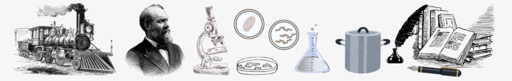
Despite these challenges, Koch tirelessly pursued his research. He utilized innovative techniques of his time, such as the agar plate and oil immersion lenses, to cultivate and study bacteria. These methods enabled him to make important discoveries and revolutionize the understanding of infectious diseases.
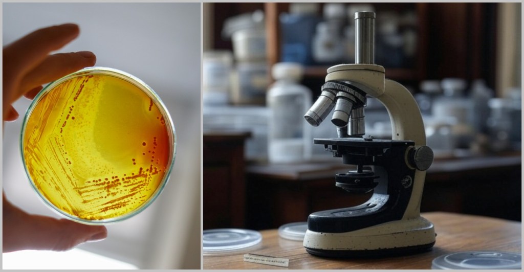
Left: An agar plate – a solid nutrient medium in a petri dish, with agar added as a gelling agent to selectively cultivate bacteria. Right: A microscope with an oil immersion lens – a special microscopy technique where a drop of oil is placed between the objective lens and the specimen to minimize light refraction, making the tiniest microbes appear sharper.
Challenges and Limitations of the Postulates
It was precisely the skepticism directed against his theories that prompted Koch to formulate the postulates in order to provide proof of a connection between the pathogenic properties of bacteria and the disease.
Koch himself recognized that his postulates do not always apply universally. A well-known example is his work with the cholera pathogen Vibrio cholerae. He discovered that this microorganism can be present not only in sick individuals but also in apparently healthy people. This finding challenged the first postulate and led Koch to abandon the universal validity of this criterion.
Koch’s Spirit of Innovation
Koch was a pioneer of his time. In his speech at the 10th International Medical Congress, he stated:
„It was necessary to provide irrefutable evidence that the microorganisms found in an infectious disease are truly the cause of that disease.”
His scientific approach of convincing skeptics through strict evidence was groundbreaking. Yet, he himself recognized that new technologies and methods were needed to answer further questions:
„With the experimental and optical aids available, no further progress could be made and it would probably have remained so for some time if new research methods had not presented themselves at that time, which suddenly brought about completely different conditions and opened the way to further penetration into the dark area, with the help of improved lens systems …”
Regarding hard-to-detect pathogens such as those causing influenza or yellow fever, he remarked:
„I tend to agree with the view that the diseases mentioned are not caused by bacteria at all, but by organized pathogens that belong to entirely different groups of microorganisms.”
Koch was already on the trail of viruses but was unable to definitively identify them due to the limited technical capabilities of his time. However, he recognized that these invisible pathogens must exist.
Why viruses break Koch’s postulates?
Koch’s research results corresponded to the scientific knowledge of his time. In the 19th century, microbiology was still in an early stage of development, where fundamental principles were just being discovered and systematically studied. Virology as an independent field emerged only after Koch’s era, when Dmitri Ivanovsky and Martinus Beijerinck discovered infectious particles smaller than bacteria. With the invention of the electron microscope in the 1930s, viruses could finally be visualized. However, viruses differ fundamentally from bacteria, which is why Koch’s postulates are often not directly applicable to them:
➤ Host dependence: Viruses can only replicate inside living host cells and cannot be grown in pure culture.
➤ Asymptomatic infections: Many viral infections occur without symptoms, making it difficult to clearly associate the pathogen with the disease.
➤ Complex detection methods: Modern molecular techniques such as PCR allow for the detection of viral genome sequences, requiring an extension of the classical postulates.
Koch and Modern Science
Robert Koch and his contemporaries laid the foundation for microbiology, particularly through the development of methods for isolating and cultivating bacteria. The germ theory of disease was a milestone in the history of science at the time. Koch understood that science is constantly evolving. If Koch had had access to modern technologies such as PCR, sequencing or electron microscopes, would he have adapted his methodology?
Modern technologies such as PCR and sequencing will be introduced in the following chapters.
His closing words at the 1890 congress provide the answer and reflect his optimism for the future:
„Let me conclude with the hope that the nations may measure their strength in this field of work and in the war against the smallest but most dangerous enemies of mankind, and that in this struggle, for the benefit of all humanity, one nation may continually surpass another in its achievements.”
If Robert Koch had been able to witness today’s advances in molecular biology, virology, and immunology, he would likely have been fascinated – not only by the new insights, but also by the revolutionary methods that make it possible to visualize even the tiniest pathogens. After all, this was precisely his motivation: to make the invisible visible, to decipher what is hidden. How might he have reacted to the first images of a virus under an electron microscope?
From the First Observations to Modern Science
What once began with dusty lenses and puzzled gazes has now become high-tech down to the molecular level. With every new technology, we peer deeper into the microcosm. Microbiology has made the invisible visible – but only modern technology allows us to truly understand the invisible. Today, we track viruses that evaded our sight for centuries.
And how we uncover the invisible today – that is the story of the next chapter.
4. Modern Methods for the Discovery and Analysis of Viruses
So far, we have familiarized ourselves with the topic of viruses. In this chapter, we shift our perspective: from wonder to measurement. Without the methods of modern biology, we would know little about viruses – their structures, their genetic material, their diversity.
What follows is a look into the engine room of science. Admittedly, a technical section – but an important one: because it is here that we see how we are able to grasp the invisible at all.
Anyone eager to understand how viruses are made visible, decoded, catalogued, and analyzed today will find here a kind of 21st-century toolbox.
But when and why do we turn to these tools?
The identification of viruses can serve different purposes: some viruses come into focus because of their impact on humans, animals, or plants, while others are discovered in environmental samples or unexplored habitats to better understand their ecological significance. The detection of known viruses is primarily used for diagnostics, whereas the identification of unknown viruses offers insights into biological diversity and evolution.
Since viruses lack universal features such as a shared cell structure, detection methods focus on their genetic material, their structure, or their interactions with host cells. The detection process does not follow a rigid scheme but instead combines various steps that vary depending on the research question and the type of virus.
The following sections will provide a detailed explanation of the key methods used for virus identification – from sample collection to bioinformatic analysis.
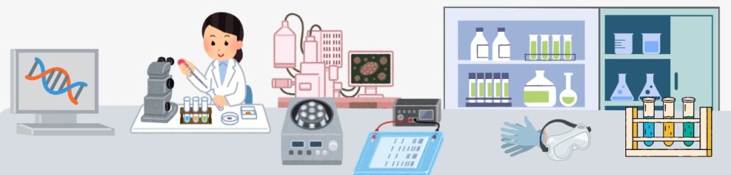
Procedures for the identification of viruses

4.1. Sample Collection
4.2. Sample Preparation
4.2. a) Filtration
4.2. b) Centrifugation
4.2. c) Precipitation
4.2. d) Chromatography
4.3. Cell Culture
4.4. Making Viruses Visible
4.4. a) Electron Microscopy
4.4. b) Crystallization
4.4. c) Cryo-Electron Microscopy
4.4. d) Cryo-Electron Tomography
4.4. e) Summary
4.5. The Genetic Fingerprint of Viruses
4.5.1. Nucleic Acid Extraction
4.5.2. Nucleic Acid Amplification
4.5.3. Sequencing
4.5.3. a) First Generation: Sanger Sequencing
4.5.3. b) Second Generation: Next-Generation Sequencing (NGS)
4.5.3. c) Third Generation: New Approaches in DNA Sequencing
4.5.3. d) Emerging Technologies: The Future of Sequencing
4.6. Bioinformatic Analysis
4.1. Sample Collection
Before we can track down viruses, we first have to find them – and that’s like a micro-scale treasure hunt, with hiding places ranging from blood to deep-sea sediment. Whether in humans, plants, or the ocean, viruses are everywhere, and researchers become detectives equipped with pipettes, protective suits, and specialized gear.
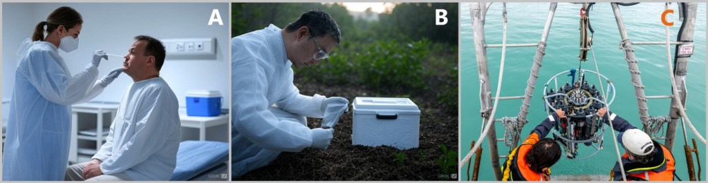
A) from humans, B) from soil, C) from marine ecosystems [Tara Oceans-Mission]
Human Samples
Who hasn’t experienced this? A swab deep in the nasopharynx – the classic method made familiar to everyone since COVID-19. But viruses don’t just hide in mucous membranes; they can also be found in blood, faeces, or tissue. Much like a thief leaves behind DNA traces, viruses reveal themselves through their genetic remnants. It is crucial that samples are collected cleanly and processed quickly – ideally as gently (and painlessly?) as possible for the patient. Plants, animals, and insects also provide sample material to investigate the presence of viruses in a wide variety of biological systems.
Environmental Samples
Water, soil, even air – viruses are everywhere. Researchers fish them out of rivers, dig them up from the ground, or capture them directly from the atmosphere using high-tech filters.
Extreme Candidates: Viruses in Extreme Conditions
In the deep sea, in eternal ice or in bubbling volcanic springs – viruses are among the toughest survival artists of all. To catch them there, special probes are needed that reach into the depths like spaceship tentacles: „Oops, what’s swimming at a depth of 4,000 metres? Just take it with you!”
More About the Ocean
Viruses play a central, often underestimated role in the health of the oceans. Wherever life exists, viruses are present – invisible yet ubiquitous players that outnumber every other biological entity. They regulate the ecosystem much like large predators, controlling populations and thus maintaining ecological balance.
An outstanding research project was the Tara Oceans Expedition (2009–2013). The goal of this four-year project was to study microbial life in the oceans and its impact on the global ecosystem. Scientists collected over 35,000 samples worldwide from plankton, algae, and viruses.
During the expedition, the research team discovered over 5,000 new RNA virus species, including the fascinating mirusviruses. These discoveries expand our understanding of the diversity, evolution, and ecology of the oceans.
If you’re interested in this expedition, check out the Tara Oceans videos – the short or the long version.
Transport: The VIP Service for Viruses
To make sure these tiny suspects don’t get damaged en route, they’re quickly put into the cold chain after collection. Deep-freeze transport and sterile packaging are a must – otherwise, the „viral loot” falls apart faster than an ice cube in the Sahara.
But a good sample is only the beginning.
What we bring home in tubes, swabs, or deep-freeze boxes is usually a biological jumble: cell debris, bacteria, proteins – and somewhere in between, a few viruses, tiny and hidden. Now it’s time to sort, clean and concentrate – before the actual analysis can even begin.
4.2. Sample Preparation
In every sample, viruses hide like needles in a microbial haystack – which is why we have to clean up before the virus hunt can begin:
- 99 % ballast: cell debris, proteins, bacteria
- 1% target: tiny virions we want to isolate
The majority of a biological sample consists of non-viral material, which makes targeted analysis extremely challenging. That’s why sample preparation is an essential intermediate step: it removes contaminants, concentrates viral particles, and prepares the material for actual analysis. The procedure varies depending on the sample type, the research goal, and the virus being investigated.
Sample preparation is like gold panning: you need patience, the right sieve – and the hope that in every bucket of sludge, there’s a nugget gleaming.
The most important techniques include:
a) Filtration
b) Centrifugation
c) Precipitation
d) Chromatography
a) Filtration – The Mega Sieve

Filtration is an initial purification step used to remove larger particles and coarse impurities.
This allows viral particles to be selectively separated from larger structures such as bacteria or cell fragments.
Function: Retains bacteria and cell debris – only virions can pass through
Special Feature: Special filters with nanopores (0.02 µm!)
Cool Fact: Some filters become electrostatically charged to catch viruses more effectively
More Information
Filtration is typically carried out using special membrane filters with defined pore sizes. Filters with a pore size of 0.2 micrometers are commonly used because they reliably retain bacteria and larger particles while allowing smaller viral particles to pass through. A practical example of this method is its use in water samples from environmental studies, where viral particles are effectively separated from other microorganisms.
An advanced variant is ultrafiltration, which uses filters with even finer pore sizes ranging from 0.01 to 0.1 micrometers. This technique not only removes bacteria but also separates smaller particles.
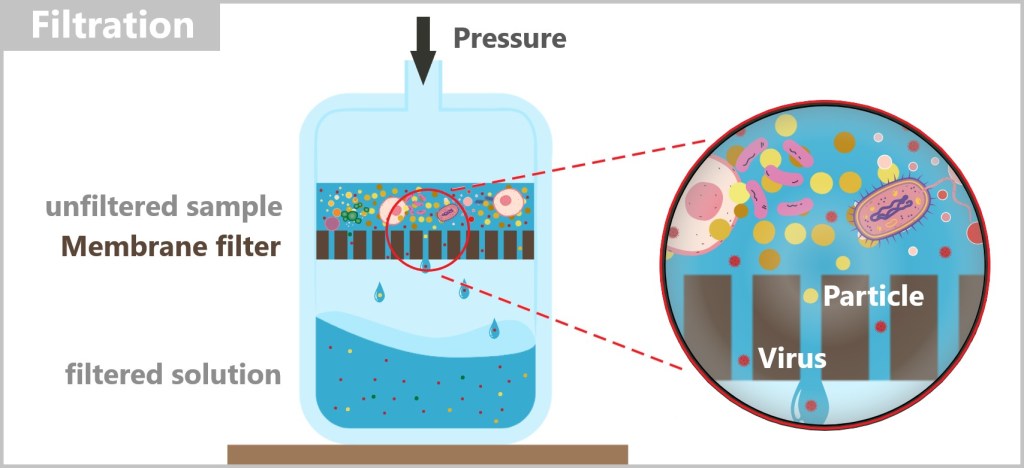
Despite its effectiveness, filtration has some limitations:
Purity: The smallest particles or dissolved substances may still remain in the sample after filtration.
Clogging: Especially in samples with a high particle concentration, the filter membrane can become blocked, complicating the process.
Capacity: The flow rate is limited by the pore size, which can make filtration time-consuming.
To obtain the purest possible virus sample, filtration is often combined with additional purification steps such as centrifugation or chromatography. These supplementary methods can remove remaining contaminants and optimize the quality of the samples for subsequent analyses.
b) Centrifugation – The Gravity Turbine

Centrifugation is a key technique for separating particles based on their size and density.
This process uses centrifugal force generated by spinning the sample at high speed.
Principle: Heavy particles sink, light ones float – viruses settle in between
High Speed: Up to 100.000 RPM (a washing machine reaches 1.200 RPM)
Trick: Density gradients can even separate different virus types from each other
More Information
How Centrifugation Works
When a solution is left standing at room temperature for an extended period, heavier particles slowly settle due to gravity. Centrifugation significantly speeds up this process by rotating the sample at speeds ranging from several thousand up to 100,000 revolutions per minute (in ultracentrifugation). The extreme centrifugal forces cause particles to separate based on their density and size.

To protect sensitive molecules from overheating, many centrifuges are equipped with cooling systems that maintain a consistent temperature throughout the entire process.
Types of Centrifugation
Differential Centrifugation
Separation principle: Particles are separated based on their size and mass. Larger and heavier particles sediment faster than smaller and lighter ones.
Procedure: The sample is treated step by step with increasing centrifugal forces. After each step, the supernatant, which contains the remaining smaller particles, is carefully transferred to a new tube. The bottom of the original centrifuge tube contains the pellet in which the larger particles have settled and is removed.
Application: This method is commonly used to isolate cell components, organelles, and viruses from complex mixtures.
A typical example of sample preparation for the investigation of unknown viruses is the extraction of a cell lysate. In this process, cells isolated from tissue samples or swabs are disrupted using chemical, physical, or enzymatic methods. This step releases viral particles that have replicated within the host cells. The cell lysate is then purified through centrifugation or filtration to separate viral components from cellular debris. Cell lysates are especially useful when there is suspicion that viruses are hidden within specific cell types or tissues.
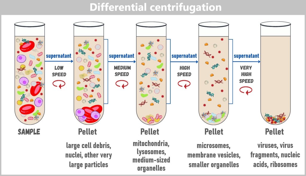
Density Gradient Centrifugation
Separation principle: Particles are separated according to their density. The sample is applied to a density gradient (usually sucrose or caesium chloride) and centrifuged. During rotation, the particles move to the position in the gradient that corresponds to their own density.
Procedure: Particles come to rest at the point in the gradient where their density matches that of the medium, enabling precise separation.
Application: This method is particularly well suited for isolating and analyzing viruses, proteins, and nucleic acids from complex mixtures.
Extraction of the Viral Fraction
After centrifugation, the viral fraction typically appears as a clearly defined layer within the centrifuge tube. This layer can be carefully extracted using a pipette to prepare the viruses for further analysis. The exact position of the viral layer depends on the method used and the physical properties of the viruses.

In most cases, the centrifuge is set to a constant speed that is sufficient to separate the particles within the density gradient. This speed is typically very high (e.g., up to 100.000 rpm during ultracentrifugation), as effective separation in the density gradient depends on generating adequate centrifugal force.
Combination of Methods
Differential and density gradient centrifugation are often combined to achieve higher purity and precision in particle separation. These methods are essential for biomedical research and diagnostics, as they allow for the precise separation and concentration of viral particles.
c) Precipitation – The Chemistry Trick

Precipitation is a well-established method for isolating and purifying virus particles from a solution.
In this process, chemical substances are added that reduce the solubility of the viruses, causing them to precipitate out of the solution.
How it works: Chemical substances make viruses heavier and sticky → they precipitate out
Advantage: Cheap and simple – but not suitable for fragile viruses
More Information
The process involves multiple steps and uses specific chemical reactions to effectively concentrate the virus particles.
Process of Precipitation
Sample Preparation: Before precipitation, the sample is often pre-cleaned – using methods such as ultrafiltration or ultracentrifugation – to remove larger particles and impurities. This improves the efficiency of the precipitation process.
Addition of a Precipitating Agent: A chemical such as polyethylene glycol (PEG), ethanol, or ammonium sulfate is added to the solution. These substances alter the chemical properties of the liquid by reducing the solubility of the virus particles.
Salting Out: In salting-out, the added salt ions or molecules compete with virus particles for the available water molecules in the solution. As fewer water molecules remain available to solvate the viruses, their solubility decreases. This leads the viral particles to aggregate and form a visible precipitate – a process known as precipitation. The surface charges and biochemical properties of the virus particles, such as size and density, favor their precipitation over other components in the solution.
Centrifugation (in the figure: ZFG): To concentrate the precipitated virus particles, the sample is centrifuged. This accelerates the sedimentation of the viruses, which collect as a solid pellet at the bottom of the tube.
Washing: The pellet is washed with a buffer or solution to remove any remaining PEG, salts or other impurities.
Result: The solution now primarily contains the isolated viruses, which can be used for subsequent analyses.
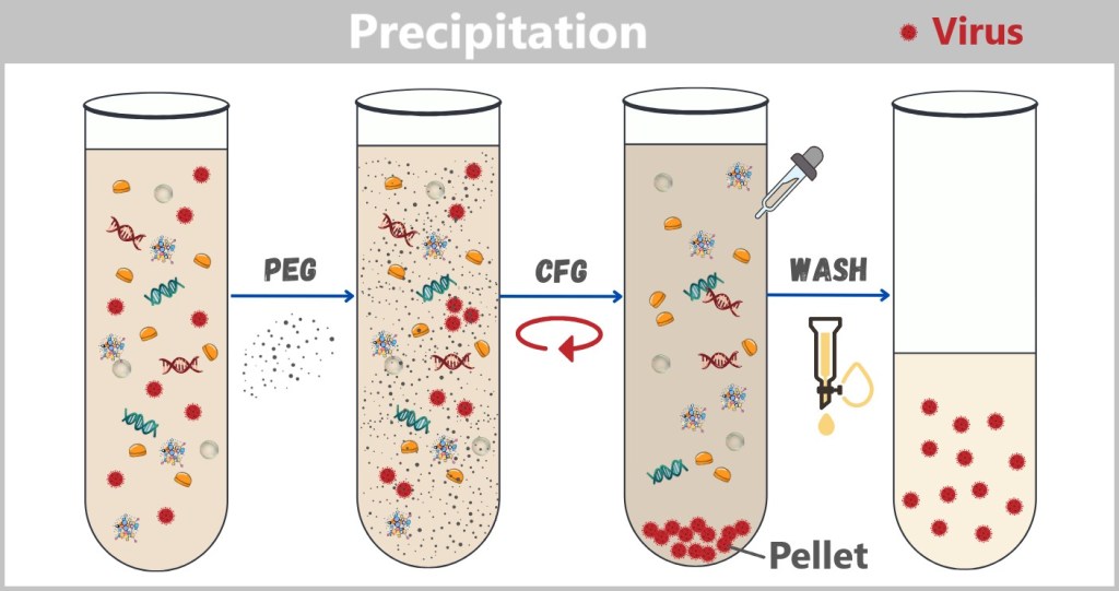
After centrifugation, the virus pellet is located at the bottom of the test tube, while the supernatant lies above. The supernatant is carefully aspirated or pipetted off to avoid disturbing the pellet. A washing solution, usually a buffer such as PBS (phosphate-buffered saline) or a similar medium, is added to the pellet. The volume of the washing solution is typically comparable to the original sample volume to effectively remove impurities. The pellet is resuspended by gentle pipetting, vortexing (light stirring with a vortex mixer), or by gently inverting the test tube so that it disperses in the washing solution. This step allows any remaining contaminants to transfer into the wash solution. After mixing, the test tube is centrifuged again, causing the viral particles to pellet once more. The wash solution (supernatant) is carefully removed without disturbing the pellet. This washing step is repeated one to three times as needed to ensure the removal of as many impurities as possible. After the final wash, the virus pellet is resuspended in a small volume of buffer (e.g., PBS or an analysis buffer) to prepare it for subsequent analyses.
Advantages of Precipitation
Widely applicable: Suitable for many types of viruses. However, it should be used with caution for very sensitive samples: especially enveloped viruses can be damaged by osmotic stress or nonspecific aggregation.
High Yield: Precipitation allows for effective concentration and purification with minimal loss of material.
Ease of Use: The process is cost-effective and does not require highly complex equipment.
Precipitation is particularly well-suited for efficiently isolating large quantities of viruses.
d) Chromatography – The VIP Lounge for Viruses
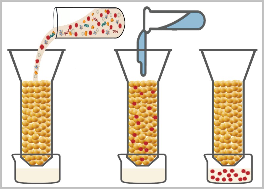
Chromatography is a highly precise purification step in virus processing.
In this method, viral particles are separated from other sample components based on their specific physical or chemical properties.
How it works: Columns separate viruses based on size, charge, or affinity
Advantage: Particularly gentle, precise and efficient
More Information
Principle of Chromatography
Chromatography is a method used to separate different substances within a mixture. In general, this process involves a mobile (moving) phase and a stationary (non-moving) phase. The mobile phase is the mixture of substances to be separated, which moves through the stationary phase, also known as the matrix. The substances in the mobile phase interact with the materials in the stationary phase. Due to these interactions, the individual components in the mixture move at different speeds or become temporarily trapped. This allows the different substances to be separated from one another.
There are various types of chromatography. One commonly used method is ion exchange chromatography, which is based on the electrical charges of the particles. This technique is particularly well-suited for purifying viral particles, as viruses typically have a defined surface charge.
Procedure of Ion Exchange Chromatography (IEC)
Controlling Viral Charge:
The isoelectric point (IEP) of a virus indicates the pH value at which the virus carries no net electrical charge. By adjusting the pH value of the surrounding solution, the electrical charge of the virus can be purposefully manipulated:
- At a pH value below the IEP, the virus becomes positively charged.
- At a pH value above the IEP, the virus becomes negatively charged.
Selection of the Matrix:
The matrix is selected to carry a charge opposite to that of the virus, allowing effective binding:
- Anion exchangers: Positively charged matrix to bind negatively charged particles.
- Cation exchangers: Negatively charged matrix to bind positively charged particles.
Typically, the matrix consists of resins or membranes that are chemically modified to carry a specific surface charge.
Binding of the Viruses:
The sample is applied to the chromatography column, and the solution flows through the matrix. The viruses bind to the matrix due to electrostatic interactions. Other molecules, such as nucleic acids or proteins, bind more weakly or pass through the column unchanged.
Washing:
Unbound or weakly bound impurities are removed from the matrix using a wash buffer. This step improves the purity of the bound viral particles.
Elution (Release of the Viruses):
To detach the bound viruses from the matrix, an elution buffer is added. This can be done in two ways:
- Change of pH value: The pH value is adjusted so that the charge of the viral particles is neutralized, causing the binding to the matrix to be lost.
- Increase in salt concentration: Additives such as sodium chloride or magnesium chloride neutralize the electrostatic binding between the viruses and the matrix.
Result:
The eluted viral particles are collected. Since impurities have already been removed during the washing steps, the eluted fraction primarily contains purified viruses, which can be used for further analyses or applications.

Other Variants of Chromatography
Besides ion exchange chromatography, there are other types used depending on the target and sample:
Affinity Chromatography: Uses specific binding between viral proteins and ligands on the matrix.
Size Exclusion Chromatography: Separates particles based on their size.
Hydrophobic Interaction Chromatography: Exploits the hydrophobic properties of the particles.
In practice, these methods are often combined. For example, a sample might first be filtered, then centrifuged, and subsequently further purified by precipitation and chromatography. The choice and sequence always depend on the type of sample and the goal of the analysis.
Why all this effort?
Simple: a bad sample gives bad data – like a blurry photo of Bigfoot. That’s why you need to work cleanly, keep things cool, and act fast… because molecules don’t forgive carelessness.
Sample preparation is not a side job – it’s the foundation. Without it, everything else falls apart. And once the viral material is well prepared, it’s time for the real deal: Now the viruses have to prove themselves – in cell culture.
4.3. Cell Culture
Viruses are the ultimate parasites: without a host cell, nothing works for them – no life, no reproduction. Alone – completely helpless. But give them a living cell and off they go. That’s why virology needs a reliable tool: cell culture. Without it, even the most dangerous virus dozes off like an office worker in the home office.
And since viruses don’t like to be alone, virologists set up a cozy home for them – a luxury shared flat in miniature: sterile petri dishes, perfect temperature, a nutrient-rich medium packed with vitamins and sugars – everything a virus’s heart desires. The cells used come from humans, animals, or plants – depending on which virus you want to pamper at the moment.
But not every virus is easy to handle. Some are demanding diva types that only thrive in specific cell lines. Others do it in anything that screams „Help!” And sometimes? Just… nothing happens. Then it’s: new cells, new luck.
Cell cultures are much more than just virus breeding stations. They enable:
➤ the replication of viruses in a controlled environment,
➤ the analysis of their properties, and
➤ the detection of infectious agents – especially with new or unknown viruses.
Why Cell Cultures Are Absolutely Cool Despite PCR
PCR tests are fast, cheap, and widely available – like the fast food of diagnostics. But they only tell you: „Yes, there was virus here!” Whether the virus is still alive and infectious? No clue!
Cell culture = reality check.
Can the virus infect cells and multiply inside them? Yes? Then we are dealing with a real pathogen. No? Then it remains genetic ghost rubbish.
Cell culture as a fitness test: indispensable when you want to:
➤ check a virus’s infectivity,
➤ test new viruses whose dangerousness is still unclear.
Viruses have to prove they’ve got what it takes first!
Even in the age of PCR and high-throughput sequencing (more on that later), cell culture remains the practical test after the theoretical exam: „All well and good – but does it actually work?”
Because only a virus that can infect cells poses a real threat. Cell culture separates the wheat (active, infectious viruses) from the chaff (harmless genetic fragments). Especially in the era of synthetic biology, this becomes crucial: just because the genetic sequence looks right doesn’t necessarily mean the virus actually works.
Infection and observation of the cell culture
Preparation of the Cell Culture
Cells are cultured in a nutrient medium that contains essential nutrients, growth factors, and a suitable pH. This environment supports the survival and proliferation of the cells. Commonly used are cell lines that allow continuous growth, such as Vero cells (derived from monkey kidney epithelial cells) or HeLa cells (human cancer cells).
The choice of appropriate host cells is based either on initial clues from microscopic observations or on testing various cell lines. Researchers often use cell lines known to support viruses from specific sample sources. For example, cell lines derived from marine organisms are commonly used for ocean samples, while human epithelial cells are preferred when studying respiratory viruses.
Infection of the Cell Culture
To detect viruses in a sample, it is applied to a suitable cell culture. If the sample contains viruses, they can enter the cells, hijack their cellular machinery for replication, and cause characteristic changes known as cytopathic effects (CPE). How such cell alterations caused by viral infections can occur is illustrated in detail in Chapter „2.8. Destruction of the Host Cell”.
Detection and Observation:
After a certain period of time, the infected cells can be examined under a light or electron microscope for cytopathic effects (characteristic changes). These effects serve as visible indications of a successful infection:
➤ Cell shrinkage or clumping
➤ Formation of syncytia (multinucleated cell aggregates)
➤ Cell lysis (disintegration of cells)

🎥 Time-lapse in real life: Tracking Influenza Virus Spread in Cell Culture
Reference to the influenza virus
The paper presents a comprehensive collection of images showing the typical cytopathic effects (CPE) following infection with the influenza virus. These visual representations illustrate the characteristic cell changes caused by the virus. However, the manual observation and evaluation of these effects is extremely labor-intensive and time-consuming. In order to optimize this process, the authors tested the use of artificial intelligence (AI), more precisely deep convolutional neural networks (CNNs), for automated image analysis.
This study impressively demonstrates how modern methods such as virology, cell biology and AI technology intertwine to develop innovative solutions to complex scientific problems.
Role and Applications of Cell Culture in Virology
Diagnosis of Known Viruses: Cell cultures are used to propagate viruses and detect their presence through specific changes in the cells.
Detection of Unknown Viruses: When the genetic or antigenic structure of a virus is unknown, cell cultures can help characterize its biological activity.
Study of the Viral Life Cycle: Cell cultures enable investigation of virus-host cell interactions, including entry, replication, and release of new viral particles.
Research on Virulence and Pathogenicity: They help to understand the mechanisms by which viruses damage cells and cause infections.
Analysis of the Immune Response: Cell cultures support the study of how the immune system reacts to viral infections and how infected cells trigger immune responses.
Testing of Antiviral Drugs: Cell cultures are used to evaluate the efficacy and safety of potential antiviral compounds and to develop new therapies.
Vaccine Production: Many vaccines, such as the measles vaccine, are produced using cell cultures.
Production of Viral Vectors: Cell cultures are essential for manufacturing viral vectors – genetically modified viruses that deliver therapeutic genes or vaccine information into cells, used in gene therapy, cancer treatment, or vaccines like those against Ebola or COVID-19 (e.g., AstraZeneca).
Limitations of the Method
Not all viruses are cultivable: Some viruses, such as Hepatitis B, require specialized cells or systems to replicate in vitro.
Viruses with very narrow host specificities: Some viruses rely on highly specific host cells, which can be difficult to reproduce in cell cultures, complicating research.
Insufficient representation of in vivo environments: Cell cultures offer only a simplified version of the natural host, which may lead to missing important virus-specific interactions or responses.
Lab-adapted viruses vs. natural viruses: Viruses that are cultured through multiple passages in cell lines may accumulate mutations that alter their characteristics. As a result, they can differ from their natural counterparts – for example, by having fewer spike proteins or altered host specificity.
Limited reproducibility of results: Cell culture conditions can influence cellular behavior, leading to variability in experimental results.
Time-consuming: Virus detection via cell culture is slower compared to molecular methods.
Complexity and cost: Establishing and maintaining cell cultures requires specialized laboratory equipment and expertise.
Biosafety risks: Working with highly pathogenic viruses requires strict safety standards, which impose additional requirements on laboratories and researchers.
Isolation and Further Processing
Cell cultures are the all-inclusive resorts for viruses – a place where they can replicate undisturbed. But, as with everything in life, even the best vacation comes to an end. For our tiny guests, it’s time to check out: „Checkout, please!” Their journey continues – straight to the high-tech labs. Now things get serious – and exciting. Because now we want to know: What exactly has grown there? And what does it look like? Welcome to the tools of virus analysis:
Selfie with the Electron Microscope: If a virus wants to know what it really looks like, electron microscopy gives it the ultimate close-up – sharper than any Instagram filter.
PCR and Sequencing: The Genetic Personality Test: A bit of genetic material here, a few enzymes there – and suddenly it becomes crystal clear who (or what) is actually sitting in that reaction tube.
ELISA: The Antibody Check: This test sniffs out antibodies in the blood – and reveals whether the immune system has already sounded the alarm. A suspicious find? Case closed!
In the next chapters, we’ll break down some of these methods – no lab coat required.
4.4. Making Viruses Visible
Viruses are like ghosts: you can feel their impact, but you never see them. They wreak havoc in cells, embed themselves in our DNA, cause diseases, shape evolution, and have been playing hide-and-seek with science for centuries. Even under the best light microscope, they remain invisible.
But as the saying goes: Seeing is believing. So how do we make the invisible visible? How can viruses be reliably detected? And how do we decode their structures and mechanisms?
The answer: we get out the really big microscopes! Devices so powerful that even the sneakiest viruses get caught red-handed – no disguise can save them. Modern imaging techniques can now dissect viruses down to the atomic level.
Welcome to the realm of modern visualization – where the invisible finally takes shape! And here we go with …
a) Electron Microscopy
b) Crystallization
c) Cryo-Electron Microscopy (Cryo-EM)
d) Cryo-Electron Tomography (Cryo-ET)
e) Summary
a) Electron Microscopy: First Images of Viruses
The history of virology began with the realization that something smaller than bacteria must be responsible for causing diseases.
The physicist Richard Feynman put it in a nutshell in 1959:
„It is very easy to answer many… fundamental biological questions; you just look at the thing!”
But how can we visualize something that lies far below the resolution limit of a conventional microscope?
The invention of the electron microscope (EM) in 1931 made this possible for the first time: viruses could be directly visualized. The method uses electron beams instead of light to reveal extremely small structures. For the first time, scientists were able to image the characteristic envelopes and shapes of viruses, thereby confirming their physical existence.
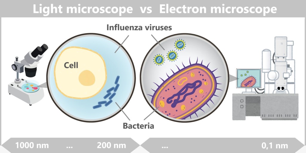
The illustration shows the differences in visualizing biological structures through two fundamental microscopy technologies.
On the left side, the view through the light microscope represents the classic capabilities used since the 17th century. Larger structures such as human cells are clearly visible here, as well as bacteria, which can be made visible through staining techniques. Viruses, however, remain invisible because their size (80–120 nm for influenza viruses) is far below the resolution limit of a light microscope.
On the right side, the view through the electron microscope demonstrates how modern technologies have overcome the limits of visibility. Not only are human cells and bacteria visible in much greater detail, but viruses can also be seen. The visualization even goes so far as to reveal high-resolution details such as the viral envelope and genome.
Light microscopes provide a general overview and enable the analysis of living cells, while electron microscopes offer deeper insights into the world of microorganisms and viruses – down to molecular details.
The following video vividly illustrates the difference between light microscopes and electron microscopes, as well as how they function.
How does electron microscopy work?
Electron microscopes have a much higher resolution than light microscopes because electrons have a much shorter wavelength than light. This allows for the visualization of structures at the nanometer scale. There are two main types:
1️⃣ Transmission Electron Microscopy (TEM)
An electron beam penetrates an extremely thin sample.
This produces high-resolution 2D images of the internal structures.
(Earlier: low-contrast spots, Today: up to 0.05 nm resolution)
Especially useful for fine details inside viruses.
2️⃣ Scanning Electron Microscopy (REM/SEM)
The electron beam scans the surface of a sample.
This produces detailed 3D images of the sample surface.
(Earlier: Rough outlines, Today: Molecular-level sharpness)
Well suited for the external structure of viruses.

(schematic representation)
Transmission Electron Microscopy: Provides a view through the virus, making internal structures visible. The virus usually appears as a two-dimensional projection with fine internal details. Electrons pass through the sample, and contrast is generated by interactions with varying densities of cellular or viral components.
Scanning Electron Microscopy: Shows a three-dimensional surface, often with a plastic, relief-like effect. The sample is scanned with electrons, producing a depth-sharp surface image. Internal structures are not visible because the electrons do not pass through the sample.
Here you can see an original TEM image of an influenza virus particle.
Further information on the use of electron microscopy
Electron microscopy (EM) enables the investigation of various aspects of the influenza virus:
🔬 Insights into the ultrastructure of the influenza virus
Using transmission electron microscopy (TEM) with negative staining, scientists have gained detailed insights into the ultrastructure of the influenza virus. The study reveals the arrangement of spike proteins (hemagglutinin and neuraminidase) on the virus surface as well as the internal structure, including the matrix protein (M1) and the RNA, highlighting differences between intact and damaged virus particles.
🔬 Insights into the Structure of Ribonucleoprotein Complexes (vRNPs)
Using electron microscopy, scientists were able to visualize the helical arrangement of the vRNPs within the virus particle. The article by Noda and Kawaoka (2010) provides a detailed description of the architecture of the vRNPs inside the virus particle and their packaging within virions. They emphasize that each of the eight vRNA segments is associated with nucleoproteins and a polymerase complex, forming the vRNPs, which are essential for the transcription and replication of the viral genome. Electron microscopic analyses have shown that these vRNPs possess a helical structure and are specifically arranged within the virion.
Electron Microscopy in Virology
Thanks to electron microscopy, viral structures and mechanisms can be uncovered, including:
✅ the shape and size of viruses (e.g., the spherical form of the influenza virus)
✅ the arrangement of spike proteins on the viral envelope
✅ and insights into the infection cycle, such as:
• how viruses enter the host cell
• how replication is initiated
Limits of Electron Microscopy
Despite its impressive resolution, electron microscopy has some drawbacks:
⚡ Sample preparation → Samples often need to be dehydrated, sectioned, and coated, which can alter their natural structure.
⚡ Samples must be fixed → meaning the sample is not examined in its natural state.
⚡ No living samples → because samples are analyzed in a vacuum to prevent electron beam scattering in air.
⚡ Radiation damage → the electron beam can alter or destroy sensitive samples.
⚡ Low contrast → biological samples often have low contrast and require special staining.
⚡ No „true” 3D image → TEM images are only two-dimensional, making it difficult to reconstruct complex structures.
Electron microscopy was the first big breakthrough: finally, viruses could be seen. But the early EM images still looked blurry – like moon photos from the 1960s. To get even closer to the viruses, more than just a microscope was needed. Atomic-level clarity was required. That’s where crystallization came into play – the ultra-HD version of virus research. Only when viral proteins are forced into perfect crystals do they reveal their molecular inner workings: atom by atom, bond by bond.
b) Crystallography: Detailed Structures of Viral Proteins
While electron microscopy could reveal the overall structure of viruses, their molecular fine structure – their atomic details – remained hidden for a long time. To understand how viral proteins are built, it was necessary to determine their atomic structure – and this was only possible through X-ray crystallography.
How did it come about?
The idea of analyzing biological macromolecules using X-ray diffraction emerged in the 1920s and 1930s. A groundbreaking breakthrough came in 1934, when physicist John Desmond Bernal, together with Dorothy Crowfoot Hodgkin, demonstrated that proteins can be crystallized in a hydrated form without losing their natural structure. This discovery was crucial for making X-ray crystallography a viable method for studying biomolecules.
In the 1930s, Wendell Meredith Stanley succeeded in isolating the tobacco mosaic virus in crystalline form. This was a milestone, as it proved that viruses are not just material particles, but are composed of regularly arranged molecules capable of forming crystals. Stanley managed to bring the virus into a solid, highly ordered structure – comparable to salt or sugar crystals. These virus crystals later enabled researchers to use X-rays to determine the atomic structure of viral proteins – marking a major breakthrough in the field of virology.
Stanley’s Breakthrough and Its Significance
How Did Stanley Perform the Crystallization?
Stanley developed an innovative method to isolate and analyze the tiny virus particles. He extracted the viruses from infected tobacco plants and purified them through centrifugation and additional purification techniques. He then dissolved the purified viruses in a solution, which he allowed to evaporate slowly. Through this process, the viruses crystallized, forming solid structures that he was able to examine more closely using an electron microscope. This marked the first step toward analyzing the structure of viruses at the atomic level.
Why Was Crystallization So Significant?
The crystallization of the tobacco mosaic virus led to two groundbreaking insights:
Proof of Viruses as Physical Particles: Until then, viruses were considered vague, invisible disease agents. Stanley demonstrated that they are physical entities with a clearly defined structure – so much so that they can even be crystallized.
Foundation for Structural Analysis: The crystals enabled later researchers to use X-ray crystallography to decipher the architecture of viruses and reveal that they consist of genetic material – either RNA or DNA – and proteins. This discovery was crucial for understanding how viruses function.
What did the structural analysis reveal?
The study of the tobacco mosaic virus showed for the first time that viruses have a clear and repeatable structure:
Genetic material and proteins: A virus’s genetic material contains the instructions for producing new virus particles, while the proteins form the protective coat and enable functions such as entry into host cells.
Distinction from other microorganisms: Stanley’s work clarified that viruses are fundamentally different from bacteria and other microorganisms. Viruses are significantly smaller, lack a cellular structure, and consist of only a minimal set of components, making them unique biological entities.
What is crystallization?
Crystallization is the physical process in which atoms, molecules, or ions transition from a disordered phase (such as a solution, melt, or gas) into a solid, ordered structure called a crystal. This transition results in the formation of a crystal lattice – a regular, three-dimensional arrangement where the particles organize themselves in a repeating pattern. During this process, the particles arrange in a way that achieves an energetically favorable state, defined by specific interactions (e.g., hydrogen bonds, electrostatic forces, van der Waals forces) and bonding angles.
Crystallization is thus the transition from chaos (disordered particles) to order (crystal lattice), driven by physical forces and energetic principles. It can occur naturally (e.g., during mineral formation) or artificially (e.g., in laboratories).
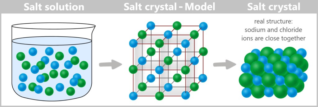
Left: In a salt solution, sodium ions (green) and chloride ions (blue) are freely moving and disordered. Right: As the water evaporates, the ions arrange themselves into a regular crystal lattice.
Basic Principle of Protein Crystallization
Protein crystallization means transforming dissolved proteins from a solution into a solid, ordered, crystalline form. The goal is to create a three-dimensional lattice in which the protein molecules are regularly arranged. This is achieved by carefully reducing the solubility of the proteins so that they slowly „precipitate” out of the solution and organize into a crystal.
The typical process is as follows:
Purification: The protein is isolated in a highly pure form, as impurities can disrupt crystal formation.
Preparation of solution: The protein is dissolved in an aqueous solution containing buffers, salts, and sometimes organic additives (e.g., polyethylene glycol, PEG).
Supersaturation: By altering conditions (e.g., evaporation, addition of precipitants like PEG or salts), the solution becomes supersaturated, causing the proteins to start precipitating.
Nucleation and crystal growth: Initially, small protein aggregates (nuclei) form, which then grow into larger crystals if conditions are favorable.
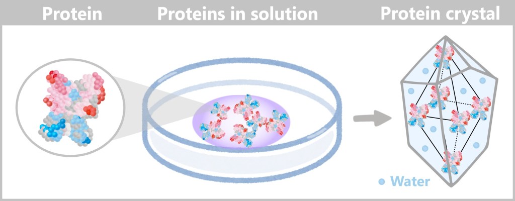
Proteins are initially dissolved in solution in a disordered state. By deliberately changing the conditions (e.g., increasing salt concentration, altering pH levels, or slow evaporation of the solvent), the solution becomes supersaturated. This causes the proteins to start organizing and grow into a crystal.
At the molecular level, proteins align into a regular lattice due to their charges, hydrogen bonds, and hydrophobic interactions. The molecules „search” for the most energetically favorable position, which leads to the formation of a stable crystal. Water molecules, represented by small blue dots, are found between the proteins. This water is an integral part of the crystal and stabilizes the protein structure through hydrogen bonding. Protein crystals often exhibit a symmetrical structure (e.g., cubic or hexagonal) because the molecules arrange themselves in repeating patterns.
Proteins are huge molecules composed of thousands of atoms, with complex 3D shapes and irregular surfaces (including charged regions, hydrophobic areas, etc.). They cannot simply be stacked alternately like sodium and chloride ions in a salt crystal.
Characteristics of Protein Crystals
The strength: Protein crystals are significantly more fragile than classic crystals like salt or diamond. They contain 30–70% water, which is trapped in channels and cavities within the crystal lattice. This makes them soft and gel-like. Mechanical stress or drying out can easily damage them.
Color: Protein crystals are usually colorless or slightly opaque (non-transparent). Proteins themselves do not have a natural color – the colorful representations in scientific illustrations are used solely to highlight structural features and chemical properties.
Selection of the Protein Crystal
During crystallization, many small crystals often form simultaneously because protein molecules start to arrange themselves at different spots in the solution. However, for analysis, only the most well-ordered crystal is selected.
How do you find the right crystal?
In the past, crystals were examined under a microscope: Clear, sharp edges and a regular shape (e.g., cubic or hexagonal) indicated high quality. Cloudy or irregular crystals, on the other hand, were less suitable.
Today, modern image analysis systems are used that combine high-resolution microscopy with automatic evaluation. Additionally, X-ray diffraction can be performed: sharp, symmetrical diffraction patterns indicate good crystal order, while diffuse or irregular reflections suggest poor quality.
Why are crystals needed?
In short: Protein crystals serve as „amplifiers” for X-rays.
A single protein molecule would produce only an extremely weak and diffuse signal during X-ray diffraction – too little to determine a detailed structure. In a crystal, however, millions of identical protein molecules are regularly arranged and oriented the same way. This causes the diffraction signals from the individual molecules to reinforce each other through constructive interference, resulting in a clear and regular diffraction pattern.
This ordered amplification is essential for X-ray crystallography, as it is only through the resulting diffraction pattern that the three-dimensional structure of the protein can be deciphered. Without crystals, analysis using this method would be impossible.
X-ray crystallography procedure
Once the protein has been successfully crystallized, its spatial structure (i.e., its precise folding and arrangement) can be determined using X-ray crystallography. This method reveals details such as:
➤ The position of each individual atom
➤ The folding structure of the protein (α-helices, β-sheets, etc.)
➤ Interactions with other molecules (e.g., antibodies, drugs)
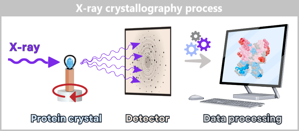
1️⃣ Shooting the X-ray beam at the crystal
A focused X-ray beam hits a protein crystal. Proteins are made up of amino acids, which in turn consist of atoms. X-rays have a wavelength of about 0.1 nm, which is on the scale of atoms, making them well-suited to reveal details at this level. The atoms in the crystal do not directly diffract the X-rays; rather, their electron clouds deflect the rays in specific directions.
2️⃣ Diffraction pattern is generated
The deflected X-rays interfere with each other and create a characteristic pattern on a detector. This diffraction pattern consists of many spots (called reflections) that appear at different positions and with varying intensity. To capture complete data, the crystal is rotated in small increments (typically 0.1–1° steps), with a diffraction image recorded at each angle.
3️⃣ Mathematical calculation of the 3D structure
The various diffraction images do not directly show the structure of the protein. Instead, they contain information about how the X-rays were scattered by the electrons of the atoms in the crystal. Using mathematical methods (Fourier transformation), these diffraction patterns are converted into an electron density map. This map reveals the three-dimensional distribution of electrons within the crystal.
Since electrons are primarily located near atomic nuclei, the positions of atoms can be inferred from the electron density map. Initially, the map appears as a „cloudy” structure, with regions of high electron density corresponding to the atoms.
The quality of the electron density map depends directly on the order within the crystal – the better the crystals, the sharper the electron density map. Through further analysis and interpretation of this map, a detailed, three-dimensional model of the protein can ultimately be constructed.
〰️ Natur Synchrotron radiation – light for nature’s smallest secrets
To examine the structure of proteins even more precisely, scientists often use synchrotron radiation – an extremely intense form of X-ray radiation generated in special particle accelerators.
💡 What exactly is it?
Synchrotron radiation is produced when charged particles (e.g., electrons) are accelerated to nearly the speed of light and then steered into a circular path by magnetic fields. In doing so, they emit high-energy radiation – including exceptionally brilliant X-rays that are ideal for protein crystallography. This allows even tiny or difficult-to-crystallize proteins to be studied in detail.
🌍 There are several major synchrotron research centers around the world, such as:
- ESRF (France) –European Synchrotron Radiation Facility
- DESY (Germany) – German Electron Synchrotron
- Diamond Light Source (UK) – Synchrotron facility in the United Kingdom
🎥 If you would like to experience live how proteins become crystals and how their structures are decoded with the help of X-rays, then join the researchers at the Diamond Light Source in the fascinating world of crystallography!
Understanding Crystallography – Part 1: From Proteins to Crystals
Here you can see how scientists transform proteins into crystals.
Understanding Crystallography – Part 2: From Crystals to Diamond
In this video, you can see how the crystals are examined using X-rays to reveal their 3D structure.
The Protein Data Bank – A Treasure of Structural Biology
X-ray crystallography has not only helped to determine the structure of individual proteins but also enabled the creation of a global resource: the Protein Data Bank (PDB). This database collects and stores the 3D structures of proteins, nucleic acids, and other biomolecules.
The PDB was founded in 1971 and today contains over 200,000 entries. Until the 1970s, X-ray crystallography was the only method for determining the three-dimensional structure of proteins at atomic resolution.
In the following decades, new techniques such as nuclear magnetic resonance spectroscopy (NMR) and later cryo-electron microscopy (Cryo-EM) expanded the range of methods. While NMR is especially suitable for small proteins in solution, Cryo-EM allows the study of large protein complexes without the need for crystallization.
Each protein structure provides detailed information about the spatial arrangement of atoms within a molecule. X-ray crystallography has not only revolutionized our understanding but has also created a global infrastructure of knowledge. A silent library where every protein tells its story – captured with atomic precision. Accessible to researchers worldwide.
X-ray Crystallography in Virology
Viruses are complex entities composed of proteins, nucleic acids (DNA or RNA), and sometimes lipids. Entire viruses are often too large and flexible to be crystallized and studied using X-ray crystallography.
However, some viruses have regular, symmetrical structures that allow for dense, repetitive packing, enabling crystallization. A well-known example is the tobacco mosaic virus, whose structure was deciphered using X-ray crystallography as early as the 1950s.
For most viruses, however, it is more practical to study individual viral proteins. Of particular interest are proteins that the virus uses to infect host cells, replicate, or evade the immune system.
To provide an example of a viral protein structure, we turn to the Protein Data Bank (PDB). The following image comes from the PDB and shows the hemagglutinin protein of the H5N1 influenza virus. Its atomic structure was determined using X-ray crystallography and deposited in the Protein Data Bank.
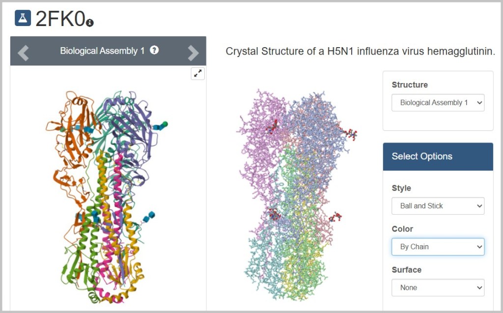
Instructions for Searching the Protein Data Bank
1️⃣ Open the Protein Data Bank (PDB): https://www.rcsb.org.
2️⃣ Search for a protein:
In our example, we are looking for the hemagglutinin protein of the influenza virus.
👉 Enter the term „influenza hemagglutinin” into the search bar.
👉 Filter the results under [Experimental Method] by selecting [X-ray diffraction].
3️⃣ Select an entry:
👉 Click on a result. For our example, choose PDB ID: 2FK0 – the hemagglutinin protein of the H5N1 influenza virus.
4️⃣ View the protein:
On the left side of the PDB page, you’ll see the cartoon representation or ribbon diagram, a schematic view of the protein’s 3D folding.
5️⃣ Visualizing the atomic structure:
👉 Click on [Structure] to switch to the 3D view.
👉 Choose a different viewer: „JSmol” (see bottom right).
👉 For the atomic structure view, select the [Style]: „Ball-and-Stick.”
🔍 Now every atom and bond is visible. You can rotate, zoom, and move the model with your mouse.
6️⃣ Highlighting structural features:
👉 Under [Color], you can choose different color schemes. For example, „By chain” colors each protein chain differently to distinguish the protein’s subunits.
Further information on the use of X-ray crystallography
For over 40 years, X-ray crystallography has been a powerful method for determining virus structures. Since we have already explored the influenza virus surface protein hemagglutinin, the following studies relate to it.
🔗 One of the first studies was published in 1981: „Structure of the haemagglutinin membrane glycoprotein of influenza virus”. It revealed the three-dimensional structure of the HA protein and laid the foundation for understanding the infection mechanisms of the influenza virus.
🔗 A more recent study from 2019 titled „Identification of a pH sensor in Influenza hemagglutinin using X-ray crystallography” investigated the binding region of the HA protein using X-ray crystallography. It showed how conformational changes in the binding region, depending on the pH level, affect the virus’s function.
🔗 A 2020 study titled „Structure of avian influenza hemagglutinin in complex with a small molecule entry inhibitor” used X-ray crystallography to elucidate the structure of the H5 hemagglutinin (HA) protein of the H5N1 influenza virus in complex with the inhibitor CBS1117. The crystal structure provided detailed insights into the molecular interactions that are crucial for the development of new antiviral drugs.
By combining the structures of individual proteins, scientists can assemble a detailed picture of the entire virus.
Limits of X-ray crystallography
Although X-ray crystallography is an incredibly powerful method for structure determination, it does have certain limitations:
⧎ Challenging crystallization: Many proteins – especially large complexes or membrane proteins – are difficult or even impossible to crystallize.
⧎ Artificial conditions: Proteins are fixed in a crystal lattice, which may not fully reflect their natural state.
⧎ Lack of dynamics: The method provides only a static snapshot and does not capture molecular motion or flexibility.
⧎ Radiation damage: The high-energy X-rays can easily alter sensitive molecules.
In Search of a New Method
These limitations made one thing clear: not every biomolecule can be forced into a crystal like Lego bricks. The solution? A microscopic flash-freeze: cryo-electron microscopy (cryo-EM). Its trick? Molecules are shock-frozen within milliseconds – so fast that water doesn’t have time to crystallize. No crystal straitjacket, no X-ray sunburn – just ice-cold atomic details.
c) Cryo-Electron Microscopy: A Modern View of Viruses
Having explored classical electron microscopy and X-ray crystallography – which first opened the door to understanding virus structures – cryo-electron microscopy, or cryo-EM for short, now leads us into a new era of research.
What is cryo-EM, exactly?
Cryo-EM is a technique in which samples are frozen extremely quickly („cryo” = cold) and then examined using an electron microscope. What makes it special is that the samples remain in an almost natural state, since they don’t need to be chemically fixed or stained as required by other methods. This makes it ideal for observing sensitive structures such as viruses.
How did it come about?
In the past, scientists had a major problem when they wanted to analyse biological samples with electron microscopes: Water evaporated in the vacuum of the microscopes and sensitive molecules were damaged by the intense electron beam. This resulted in blurred or distorted images.
Researchers had already come up with the idea of cooling samples to protect them. But there was another problem: when water freezes, it forms ice crystals. These crystals scatter electrons so strongly that capturing clear images became impossible.
The crucial breakthrough came in the 1980s, when scientist Jacques Dubochet developed a technique called plunge freezing. In this method, the sample is cooled extremely rapidly to very low temperatures – so fast that ice crystals don’t have time to form. Instead, the water solidifies into a glass-like, frozen state that perfectly preserves the biological sample. This marked the birth of cryo-electron microscopy (cryo-EM).
Another major advancement came in the 1970s, when Joachim Frank developed a method to improve the blurry images produced by electron microscopes using computer-based calculations. By combining numerous images of individual molecules taken from different angles, he was able to reconstruct a sharp 3D model. This made it possible, for the first time, to determine the structure of biomolecules without the need for crystallization – a significant advantage for proteins that are difficult or impossible to crystallize.
In 1990, Richard Henderson used cryo-EM for the first time to study a biomolecule at such high resolution that even small details like amino acid side chains became visible. For these groundbreaking developments, Dubochet, Frank, and Henderson were awarded the Nobel Prize in Chemistry in 2017.
Since then, the technology has advanced rapidly:
↗️ Modern cameras capture razor-sharp images directly, without loss of quality.
↗️ Automated microscopes can analyze multiple samples simultaneously.
↗️ Powerful computer programs enable the processing of massive amounts of data to calculate even more precise structures.
Thanks to these advances, cryo-EM can now visualize complex molecules, proteins, viruses, and even entire cell structures in their natural state – with unprecedented levels of detail.
Next, we’ll take a closer look at how cryo-EM makes viruses visible.
Making Viruses Visible with Cryo-EM – Step by Step
1️⃣ Sample Preparation: Growing and Isolating Viruses
To study viruses, you first need to have them. They are usually grown in suitable host cells, such as cell cultures in the lab. Viruses are parasites that can only reproduce inside host cells. To study them, you infect appropriate cells in a culture and allow the viruses to multiply.
After infecting the cells, the viruses are „harvested” at specific time points to study different stages of their life cycle (e.g., attachment, entry, replication). The viruses are then isolated and purified from the cell culture – using methods like centrifugation or filtration – to obtain a clean virus sample free of interfering cell debris.
2️⃣ Sample Preparation: Applying the Sample to a Grid
The purified virus sample is a watery solution in which the viruses are suspended. This virus solution is applied with a pipette onto a grid (see the image below).
A typical cryo-EM grid is tiny, about 3 millimeters in diameter, so it fits into the electron microscope’s holders. The grid is made of a fine metal mesh (e.g., copper or gold) that looks like a sieve. An ultrathin carbon foil with tiny holes – usually 1 to 2 micrometers in diameter – is placed on the metal mesh. Due to surface tension, the virus solution spreads into these tiny holes and sticks there before freezing. This setup serves two important purposes: the grid provides stability, while the holes allow the electron beam to pass through freely, minimizing background noise.
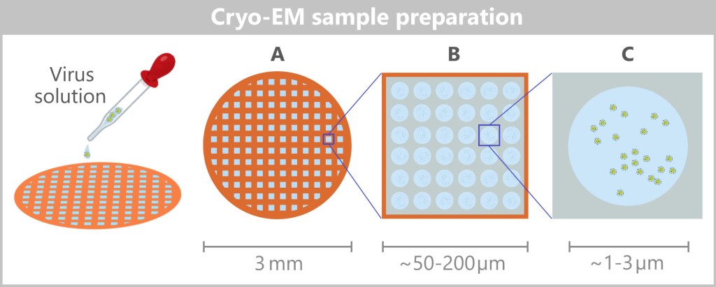
A – Grid covered with a perforated carbon film,
B – Enlarged image of a grid opening, called a mesh hole,
C – Enlarged image of a hole where the viruses adhere
3️⃣ Rapid Freezing of the Sample
The sample – or the grid – is now flash-frozen by plunging it into liquid ethane or nitrogen at around –180 °C. This process is called vitrification – the water doesn’t form crystals but instead turns into a glass-like state that perfectly preserves the structure. This keeps the viruses in their natural state, as if frozen in time. Additionally, the ice protects the molecules from damage caused by the intense electron beam.
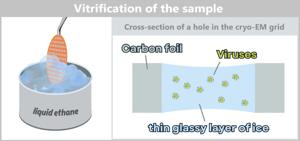
4️⃣ Imaging in the Electron Microscope
The frozen grid with the viruses is placed into the cryo-electron microscope. In the vitrified solution, the viruses are randomly oriented – they are positioned at various angles. The electron beam hits the sample from a fixed direction (usually perpendicular), and a highly sensitive camera captures 2D projections of the viruses.
Because each virus is frozen in a different orientation, images are automatically captured from many different angles – without needing to rotate the grid. This large number of images is crucial for the later 3D reconstruction. In total, often thousands to hundreds of thousands of images are taken.
5️⃣ Data Processing: From 2D Images to a 3D Model
After image acquisition, the real challenge begins: computational reconstruction. Specialized software identifies individual virus particles in the 2D images and sorts them according to their orientation.
Using mathematical methods such as „Single Particle Analysis”, the 2D images are combined to compute a high-resolution 3D model of the virus. The more images and the better their quality, the sharper the model becomes.
If different stages of the virus life cycle are to be studied (e.g., before and after entering a cell), this process is repeated with samples taken at different time points. This way, changes in the structure over time can even be visualized.

The following videos provide a clear summary of the information about cryo-EM covered so far:
🎥 What is Cryo-Electron Microscopy (Cryo-EM)?
🎥 Cryo-EM Animation
6️⃣ Interpretation and Visualization
After the 3D reconstruction, a high-resolution model of the virus is available, showing its structure – such as the envelope, spike proteins, and sometimes even internal structures.
Now it’s time to analyze, interpret, and visually present the icy data. This step is crucial for deciphering the biological significance of the structure and making the findings accessible for further research or public understanding.
Interpretation and visualisation steps
a) Structure Analysis: Scientists examine the 3D structure to identify key features of the virus or its proteins. This analysis helps to understand the molecular mechanisms of viral infection. This includes, for example:
- Binding sites: Where does the virus attach to host cells?
- Functional regions: Which parts of the protein are essential for infection or replication?
- Structural variations: Are there differences in the structure between different virus strains or life cycle stages?
b) Comparison with Known Structures: The reconstructed structure is compared with previously known structures from databases such as the Protein Data Bank (PDB). This can provide insights into evolutionary relationships, functional similarities, or potential targets for drug development.
c) Visualization of the Structure: Using specialized software, the 3D model is visualized to clearly present the structure and highlight important features. Various forms of representation are used, such as:
- Surface representation: Shows the external shape of the virus or protein.
- Ball-and-stick model: Displays the arrangement of atoms and bonds.
- Secondary structure: Highlights structural elements such as α-helices and β-sheets.
d) Publication and Data Sharing: The results are published in scientific journals – often accompanied by high-resolution images or animations of the 3D structure. In addition, the raw data and reconstructed models are stored in public databases such as the PDB (Protein Data Bank) or the EMDB (Electron Microscopy Data Bank), allowing other researchers to access and build upon the findings.
If viruses knew how often we can now rotate and zoom in on them in 3D… they’d put some clothes on!
Influenza Virus in 3D: An Example
It can be challenging to find 3D models of viruses online. Research data is often released only after studies are published and then stored in specialized databases like the EMDB (Electron Microscopy Data Bank). However, this data is difficult for non-experts to access, as it requires specialized software to view it as 3D models.
Fortunately, the NIH 3D platform (National Institutes of Health) offers a helpful example: a 3D model of an influenza virus created using cryo-electron microscopy. You can view it via this link! Please note that you may need a 3D viewer to explore it.
Further information on using the cryo-EM
🔬 This study on the influenza virus used cryo-electron microscopy to reveal the interactions between the nucleoproteins and the viral RNA as well as the specific arrangement of the ribonucleoprotein complexes (RNPs) within the virion. Such structural insights are crucial for understanding the mechanisms by which the influenza virus packages its genome and replicates during the infection cycle.
🔬 Additionally, an earlier study by Liu et al. (2017) revealed structural details of filamentous influenza virus particles and their RNP organization using cryo-EM.
Why Cryo-EM Is So Brilliant – Especially for Viruses
Cryo-EM is an unbeatable tool when it comes to visualizing viruses – especially those tricky, hard-to-capture candidates:
- Viruses with their tricky spike proteins
- Huge protein complexes that refuse to crystallize properly
- Membrane proteins that otherwise just say „Hello!” and fall apart immediately
The method: It freezes viruses in the blink of an eye, preserving them like in a time capsule, and produces thousands of images using an electron beam. A computer then assembles these images into a high-resolution 3D model – allowing us to see exactly how a virus is structured. This approach is called Single Particle Analysis (SPA) because individual virus particles are analyzed and computationally combined into a 3D structure.
From Still Frames to Blockbusters
What cryo-EM delivers in detailed „snapshots” is impressive – but sometimes one picture just isn’t enough. To understand how viruses move, hijack cells, or replicate, you need moving scenes. This is exactly where cryo-electron tomography comes in: a technique that lets you watch viruses at work almost like in a movie.

d) Cryo-Electron Tomography – 3D Virus Models Inside the Cell
While cryo-EM examines highly purified, isolated viruses, cryo-ET allows scientists to capture three-dimensional snapshots of molecular interactions directly within the cell. This makes it possible to visualize viruses in their natural environment – inside the cell.
Making Viruses Visible with Cryo-ET – Step by Step
1️⃣ Sample Preparation – Freezing the Cell
Suitable cells are grown in cell culture and infected with viruses. After waiting for a defined time point – for example, when the viruses enter the cell or begin replicating – the cells are harvested. They are then transferred into a buffer solution to create a homogeneous cell suspension.
The cell suspension is then applied to a cryo-EM grid – a small metal grid with a perforated carbon film, already familiar from cryo-EM techniques.
The grid is immediately plunged into liquid ethane or liquid nitrogen (at around -180 °C). This rapid freezing technique, known as vitrification, preserves the cellular structures without the formation of disruptive ice crystals.

2️⃣ Thinning cellular areas (if necessary)
Vitrification stabilizes the cells – they are now rigid like glass. Since cells are often too thick for cryo-ET, scientists use a Focused Ion Beam (FIB) to thin the ice layer down to the desired thickness.
This is how it works: The cryo-EM grid is first scanned in a FIB-SEM device (Focused Ion Beam combined with Scanning Electron Microscope) to locate interesting cells. Then, a focused ion beam precisely mills a thin lamella (~100–200 nm thick) from the ice layer. This lamella represents a cross-section of the cell and reveals relevant areas containing virus particles – for example, the cell membrane or the cytoplasm with viruses.
Here’s how it looks in practice: the video titled „Cryo-lamella preparation” in the section „FIB-milling of lamella in waffle grids” on the page „Cryo EM 101, Chapter 3” demonstrates the process.
3️⃣ Image acquisition in cryo-EM
The frozen cell grid is placed into the cryo-electron microscope. Here, an electron beam generates high-resolution images of the sample.
Tomography – Like a CT scan for cells
The sample is gradually rotated. A goniometer (rotating mechanism) tilts the grid in small angular steps (e.g., 1–2°), typically over a range of ±60° to ±70°. For each angle, a 2D image is taken, creating a so-called „tilt series” – a collection of 2D images from different perspectives (see illustration below).
📌 Cryo-ET vs. SPA: Unlike Single Particle Analysis (SPA), which requires many identical viruses, Cryo-ET focuses on a specific area of the sample – often a single cell or a virus-host cell interaction. This means there is no need for a large number of identical particles; instead, individual biological structures can be studied directly in their natural environment.
4️⃣ 3D Reconstruction
Cryo-ET uses the tilt series to computationally reconstruct a 3D model – like a medical CT scan, but for viruses instead of bones. The result is a hologram-like volumetric image that shows how viruses dance, dock, and trick inside real cells.
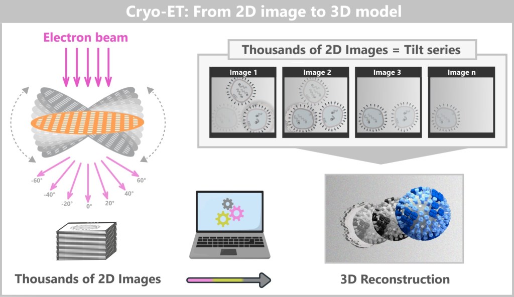
5️⃣ Interpretation & Visualization
Now things get exciting! The 3D models show viruses in their natural environment:
- how they sit inside the cell
- how they interact with cellular organelles
- different stages (e.g., entry, replication, release)
The results are interpreted to understand, for example, the virus’s infection mechanism or its interaction with the host cell.
Sometimes multiple time points are compared to create a kind of „movie” that simulates the dynamics.
The following video gives an impression of this: detailed 3D models of an influenza virus during budding at the cell membrane were visualized and then compiled into a film.
6️⃣ Publication and Data Storage
To make the spectacular virus models accessible to everyone, they are deposited in public databases like the Electron Microscopy Data Bank (EMDB) – the Netflix for structural biologists.
Why that’s cool:
- Open Science = No scientist has to reinvent the wheel twice.
- Transparency = Everyone can see exactly how the „movie” was made.
- Collaboration = Teamwork makes virus research a hit too.
If viruses had Twitter, they’d be trending now with #EMDBChallenge.
Further information on using cryo-ET
🔬 The study „Quantitative Structural Analysis of Influenza Viruses Using Cryo-Electron Tomography and Convolutional Neural Networks” utilized cryo-electron tomography (cryo-ET) and modern computational techniques to investigate the structure of the influenza virus. It reveals the diverse shapes of the virus and includes videos from 3D reconstructions that illustrate the process.
🔬 The study „Structural Changes in Influenza Virus at Low pH Characterized by Cryo-Electron Tomography” investigated how the influenza A virus responds to acidic conditions it encounters during entry into host cells. Using cryo-electron tomography, the researchers observed that at low pH-value, the viral envelope proteins (hemagglutinin) undergo structural changes that lead to the fusion of the viral and cellular membranes. This fusion enables the virus to release its genetic material into the host cell and initiate infection.
Researchers are not only investigating human pathogenic viruses
Researchers are no longer interested only in pathogens like influenza or coronavirus – environmental viruses are equally fascinating. Chief among them are bacteriophages, viruses that infect bacteria. In the oceans, they act as true ecological engineers.
1️⃣ Tiny directors in the ecosystem
Phages specifically kill certain bacteria, keeping the microbial balance in the ocean stable. In doing so, they indirectly regulate important cycles such as the carbon and nitrogen cycles. Understanding their structure and behavior helps us better grasp how stable marine ecosystems function.
2️⃣ Experience evolution live
Phages are the most abundant biological „organisms” on Earth – and genetically incredibly diverse. Using cryo-EM, researchers are constantly discovering new virus families. Their genetic codes end up in databases, telling a story about the co-evolution of viruses and bacteria.
3️⃣ From the sea to the lab
Some marine phages produce enzymes with real potential: for genetic engineering, diagnostics, or even as alternatives to antibiotics. They could also help in agriculture by targeting harmful bacteria – without the use of harsh chemicals.
4️⃣ And where do the data go?
Structural and gene sequences are made openly accessible – for example, in the NCBI Virus Database or the EMDB. Bioinformaticians explore these databases to discover new genes, clever mechanisms – and sometimes ideas for the next biotechnological innovation.
Limits of cryo-EM
Cryo-EM (including Single Particle Analysis (SPA) and Cryo-Electron Tomography (Cryo-ET)) are groundbreaking techniques, but they also have some limitations that depend on technical, biological, and practical factors:
Sample preparation is challenging
Problem: The samples must be extremely thin (only a few hundred nanometers) and perfectly vitrified without ice crystals, which could damage the structure. This is technically difficult and requires a lot of expertise.
Impact on viruses: If the virus solution is not frozen evenly or is too thick, the images can become blurry or the viruses may be damaged. In cryo-ET, thick cell samples can scatter the electrons too much, which worsens the image quality.
Limited resolution
Problem: Although cryo-EM can deliver very high-resolution images (up to 2–3 Ångström under optimal conditions), the resolution depends on the quality of the sample and the amount of data. For complex or variable structures (e.g., flexible viruses), the resolution can suffer.
Impact on viruses: The tiniest details (e.g., individual atoms in proteins) are not always visible, especially when viruses are moving or have variable shapes.
Limited dynamics: frozen in time
Problem: As impressive as the 3D models are, they always show just a frozen moment in time. Real movements or processes – like a virus entering a cell live – remain out of reach.
Impact on viruses: With Single Particle Analysis (SPA), we only see one structure at a specific moment in time. Even with Cryo-ET, researchers must freeze different cells at various „stages” of infection to reconstruct a timeline. It sounds like a movie – but it’s more like stop-motion reconstruction than a live stream.
High costs and complexity
Problem: Cryo-EM requires expensive equipment (electron microscopes cost millions), specialized laboratories (e.g., vacuum and cryo conditions), and a lot of computing power for data analysis. This makes the method time-consuming and costly.
Impact on viruses: Only well-equipped research institutions can use cryo-EM, which limits access. Small labs or developing regions often cannot apply this technique.
Noise and Data Volume
Problem: The images are often noisy because only a limited number of electrons are used to avoid damaging the sensitive samples. Processing requires thousands of images, which is computationally intensive.
Impact on viruses: If the amount of data is insufficient or the noise level is too high, the 3D models can become inaccurate.
Limited sample size
Problem: Cryo-EM only works with very small samples (e.g., individual viruses or cells). Larger structures like whole tissues are difficult to study because the electrons cannot penetrate deeply enough.
Impact on viruses: Cryo-ET can image cells, but only up to a certain thickness (about 1 micrometer). Larger organisms or tissues are not suitable for this technique.
Sources
Cryo Electron Microscopy: Principle, Strengths, Limitations and Applications
Challenges and triumphs in cryo-electron tomography
e) Summary
Science has developed increasingly powerful methods over decades to make the world of viruses visible. While the naked eye and light microscopes quickly reach their limits, electron microscopy, X-ray crystallography, and finally cryo-EM and cryo-ET have provided entirely new insights. These technologies have revolutionized our understanding of viruses.
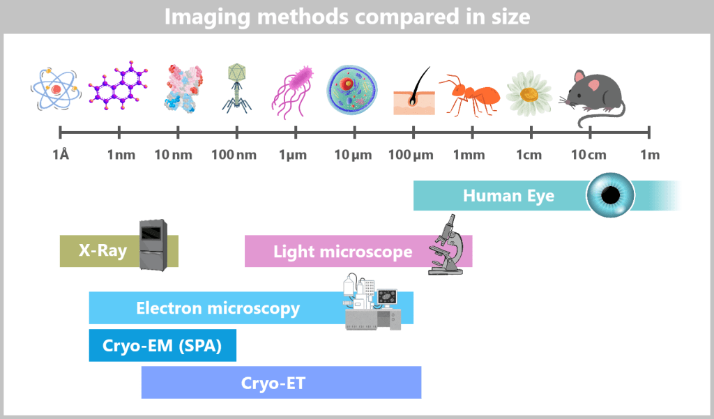
Scaling of Imaging Techniques
➡️ Human Eye
Visible range: approx. 0.1 mm (100 µm) to several meters
Example: Hair, grain of sand
➡️ Light Microscope
Visible range: approx. 200 nm – 1 mm
Example: Bacteria, cells, cell nuclei
➡️ Classical Electron Microscopy (EM, TEM/SEM)
Visible range: approx. 0.2 nm – 100 µm
Example: Viruses, cell organelles, cell membranes
➡️ X-ray Crystallography
Visible range: approx. 1 Å (0.1 nm) – 10 nm
Example: Atomic structures of proteins
➡️ Cryo-EM (Single Particle Analysis)
Visible range: approx. 2 Å (0.2 nm) – 100 nm
Example: Protein complexes, ribosomes
➡️ Cryo-ET (Cryo-Electron Tomography)
Visible range: approx. 3–5 nm – 200 µm
Example: Viruses inside cells, cell organelles at high resolution
Electron Microscopy (1930s)
→ First Images of Viruses
Electron microscopy (EM) was a revolutionary advancement in microscopy because it allowed imaging of structures far below the resolution limit of light microscopes for the first time. Instead of light, EM uses a beam of electrons, which enables much higher resolution. This enabled scientists to visualise viruses that are too small to be viewed with conventional microscopes for the first time.
EM was a major breakthrough, but its limitations in depicting samples in their natural state and the lack of 3D information led to the development of X-ray crystallography.
X-ray crystallography (1950s–present)
→ Detailed structures of viral proteins
X-ray crystallography made it possible to decipher the atomic structure of proteins and other biomolecules. In this method, a crystal of the protein is irradiated with X-rays, and the resulting diffraction pattern is analyzed to determine the positions of the atoms. This technique provided detailed insights into the structure of viral proteins, which was crucial for understanding their function and for drug development.
Although X-ray crystallography is powerful, its limitations in studying large, complex structures and the need for crystals led to the development of cryo-electron microscopy (cryo-EM).
Cryo-EM (1980s–present)
→ A modern view of viruses
Cryo-EM combines the advantages of electron microscopy with gentle sample preparation. Samples are rapidly frozen (vitrified), preserving them in a near-native state. This allows imaging of individual virus particles or large protein complexes without the need for crystallization. Cryo-EM delivers high-resolution images and can also capture flexible or dynamic structures.
Cryo-EM was a major breakthrough, but it was limited to isolated particles and could not image complex cellular environments. This led to the development of cryo-electron tomography (cryo-ET).
Cryo-ET (2000s–present)
→ 3D virus models inside cells
Cryo-ET expands on cryo-EM by creating 3D models of virus particles or other structures directly within their cellular environment. The sample is imaged from different angles, and the images are combined into a 3D model. This allows viruses to be studied in their natural context, for example, how they interact with cells or replicate.
Cryo-ET is a powerful tool, but its limited resolution and the complexity of sample preparation could drive the development of new technologies that enable even higher resolutions in complex cellular environments.
Each of these technologies has expanded the limits of our vision – while simultaneously introducing new challenges. Yet it is precisely these limits that have driven the development of even more powerful methods. Science is a continuous process of discovery, refinement, and pushing boundaries.
They say, „Seeing is believing”, but for biologists, „Seeing is understanding”. The more detailed we can map biological structures, the deeper we penetrate into the mysteries of life. But simply visualizing a virus and its interaction with the host is not enough to fully decipher its nature.
From Seeing to Decoding: The Next Level of Knowledge
To understand what truly defines a virus, we must decode its genetic legacy – its unique „fingerprint”. This is achieved through modern molecular biology techniques that analyze the viral nucleic acids, providing a glimpse into the virus’s genetic blueprint.
4.5. The Genetic Fingerprint of Viruses
Once viruses had finally become visible – thanks to electron microscopy and crystallographic analysis – the next big question emerged: What actually makes a virus a virus?
It quickly became clear: like any biological system, viruses also need a genetic blueprint – something that encodes their characteristics and enables their replication. But what exactly carries this information?
For a long time, protein was considered the prime candidate: diverse, complex, and seemingly perfectly suited. DNA, on the other hand, appeared to many researchers as too simple, too monotonous to be the carrier of life.
But as it turned out, the answer lay precisely there: in this inconspicuous molecule that proved to be the ultimate data carrier of life – and, in the case of some viruses, in its close relative, RNA.
The discovery that it wasn’t proteins but nucleic acids that hold the key to viral replication was a scientific thriller in its own right – marked by misconceptions, rival research teams, and groundbreaking revelations.
Searching for the code of life
Early Approaches to Decoding Heredity
The foundations of genetics were laid in the 19th century through Gregor Mendel’s experiments. Scientists recognized that organisms pass on their traits to the next generation, but the exact mechanism remained unclear for a long time. By the late 19th century, researchers had identified chromosomes within cells as possible carriers of hereditary information and began searching for the key molecules responsible. Due to their complexity, proteins seemed the most likely candidates.
Wendell Meredith Stanley and the Tobacco Mosaic Virus
In the 1930s, the work of Wendell Meredith Stanley confirmed the central role of proteins in the structure of viruses. Stanley isolated the Tobacco Mosaic Virus and processed it in an innovative way: he extracted the virus from infected tobacco plants, purified it through centrifugation, and then crystallized it from solution. These crystals contained both proteins and genetic material, but at first, the research focused solely on the protein. It was assumed that the protein carried the genetic instructions required for virus replication.
The Paradigm Shift: From Proteins to DNA
Doubt surrounding the protein hypothesis grew when, in 1944, Oswald Avery demonstrated that DNA has the ability to transform the properties of bacteria. In his experiment, DNA was extracted from one bacterial strain and transferred to another, revealing that DNA can carry genetic information. However, this discovery was initially met with skepticism.
It was the Hershey-Chase experiment of 1952 that provided the decisive breakthrough. Scientists Alfred Hershey and Martha Chase worked with bacteriophages – viruses that infect bacteria. They radioactively labeled the DNA of the viruses and traced its path into the host cells. The protein shells of the phages remained outside the cell, while the DNA entered and directed viral replication. This conclusively proved: DNA – not protein – is the carrier of genetic information.
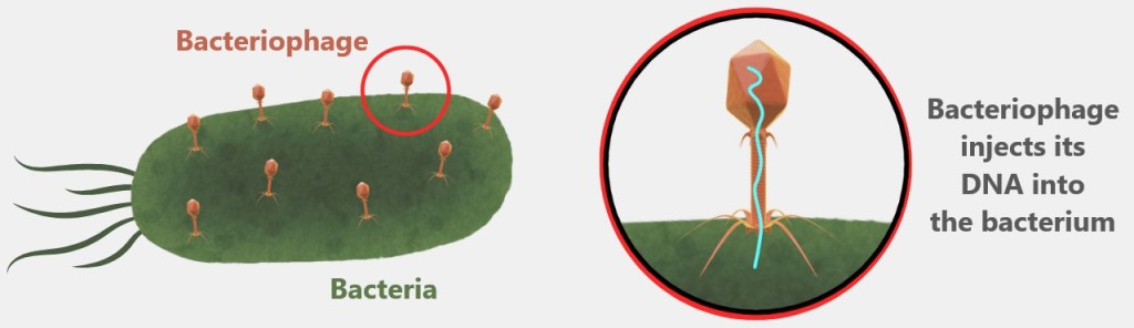
The Double Helix and the Role of RNA
In 1953, James Watson and Francis Crick unraveled the structure of DNA, aided by Rosalind Franklin’s X-ray diffraction images. The discovery of the double helix revealed how DNA stores genetic information and replicates during cell division. Around the same time, it became clear that RNA carries the genetic material in some viruses, including the tobacco mosaic virus. This cast Stanley’s earlier work in a new light: the RNA inside the virus particles – not the protein – was the true carrier of genetic information.
Viruses – The Minimalists Among Life Forms
Viruses are true masters of reduction. These minimalist survivors have perfected the art of genetic efficiency – whether with DNA, RNA, or even reverse-transcribed RNA (like the negative single-stranded RNA of influenza viruses, which is essentially a mirror image).
Their genome is like an ultra-light survival backpack:
✔ All the essentials that count – blueprints for replication, packaging, host hijacking
✖ No ballast – no ribosomes of their own, no energy production, no small talk
Viruses are genetically unique: while all known living organisms use only DNA as their genetic material, viruses can use either DNA or RNA – a fundamental difference that drives their remarkable adaptability and evolutionary creativity.
Key Molecular Biology Methods for Viral Genome Analysis
Thanks to modern molecular biology techniques, viruses can now be analyzed with high precision. This allows scientists to:
- decipher their genetic information,
- trace their evolutionary origins, and
- track their transmission pathways.
Depending on the research question, different methods are used:
- Is the goal to identify a virus?
- Should its genome be fully sequenced?
- Or is the aim to observe its activity within the host system?
The following sections present the key methods used to analyze the genetic fingerprint of viruses – from isolating the genetic material to modern sequencing technologies.
4.5.1. Nucleic Acid Extraction
4.5.2. Nucleic Acid Amplification
4.5.3. Sequencing
💡Note: For basic information on DNA and RNA and their functions, we recommend Chapter „4.2. The Protein Biosynthesis” in the publication „The Wonderful World of Life”. It clearly explains the fundamentals and provides an ideal foundation for understanding this topic.
4.5.1. Nucleic Acid Extraction
To analyze a virus in detail, we must first reach its innermost treasure: its genetic material – DNA or RNA must first carefully extracted. However, the nucleic acid is well hidden, wrapped in protein envelopes, embedded in cell debris or mixed with all kinds of molecular ‘by-catch’.
The task: to free the viral nucleic acid from this molecular jumble – cleanly, efficiently, and without causing any damage.
The goal: to obtain as much pure DNA or RNA as possible – ready for PCR, sequencing, or mutation analysis.
Nucleic acid extraction is therefore the first and one of the most important steps in any molecular virus diagnostics. Depending on the sample type, virus species, and the purpose of the analysis, different extraction methods are used – ranging from classic kits to automated high-throughput systems.
How does nucleic acid extraction work?
The process can be divided into four simple steps:
1️⃣ Cell lysis – Breaking everything up first
Before accessing the RNA or DNA, the cells (and possibly viruses) in the sample need to be broken up. This can be done, for example, by ultrasound, enzymes, or mechanical grinding. The main goal is to remove the outer shell so that the genome is exposed.
Methods that get to the core
Ultrasound: Sonication breaks down cell and viral envelopes using sound waves.
Enzymes: Proteinase K degrades proteins that package the genome.
Mechanical grinding: Small glass beads in a tube are shaken. The beads collide with the cells and tear the cell membrane apart.

Intact structure (left): A schematic representation of an intact cell with organelles, nucleus, and DNA. Inside the cell, influenza viruses are visible. Additionally, a single influenza virus is shown enlarged, with its spherical envelope consisting of a host cell membrane, a capsid, and RNA strands.
Cell lysis (middle): The cell membrane is shown perforated, allowing the cytoplasm to leak out. The nuclear membrane also has holes. An influenza virus is depicted enlarged with a broken envelope, releasing viral RNA and other components. Next to the cell, symbols for chemical substances (bottle), physical forces (sound waves), and mechanical forces are illustrated to represent the different methods of cell lysis.
Contents released (right): After cell lysis, the organelles, DNA, and other cellular components float freely in the medium. Also visible are the released components of the influenza virus, including RNA segments, spikes, and other molecular components, which are shown in the enlarged view.
2️⃣ Cleanup – Fishing out proteins & co.
At this stage, the sample is quite a mix: nucleic acids, proteins, fats, and cell debris are all jumbled together. To ensure that only what we need remains in the end, reagents or enzymes are used to specifically break down all the excess material.
Methods that clear things up
Phenol-chloroform extraction: Old but reliable – effectively separates nucleic acids from interfering proteins and lipids. Especially useful for heavily „contaminated” samples.
👉 Caution: The chemicals used are quite toxic – only for experienced hands (and with safety goggles!).Proteinase K: This enzyme breaks down proteins such as membrane or structural proteins that are still floating around in the sample – ensuring that the DNA/RNA remains undisturbed.
DNase/RNase treatment: Used to specifically degrade non-viral DNA or RNA – especially useful when, for example, only viral RNA is to be analyzed.
3️⃣ Purification – Pure RNA or DNA
Now it gets elegant: the nucleic acids are selectively bound – to special surfaces like silica membranes or magnetic beads. The rest? Simply washed away. It’s like a molecular sieve – just smarter.
Methods that filter properly
Spin columns (column-based method): DNA or RNA binds to a special membrane, usually made of silica. Then it’s all about rinse, rinse, rinse – until everything else is gone. What remains in the end: beautifully pure nucleic acid. This method is fast, reliable, and found in many lab kits.
Magnetic bead technology: Tiny magnetic beads selectively bind to nucleic acids. Using a magnet, the right matches are quickly fished out of the mix. It’s lightning-fast and perfectly suited for automated high-throughput processes that need to handle thousands of matches per hour.For more information, see the videos:
DNA and RNA extraction with magnetic beads – How it works and
Nucleic acid purification with chemagic M-PVA Magnetic Bead Technology.
4️⃣ Elution – The grand finale
Now comes the final act: the purified nucleic acids are dissolved in a small volume of liquid (elution buffer or water) – and voilà: the sample is now ready for analysis. Free of any clutter, but full of potential for PCR, sequencing & more.

Left: The released cellular and viral contents after cell lysis, consisting of a mixture of cell components, proteins, and nucleic acids.
Middle: After the removal of proteins and impurities, only the nucleic acids (viral RNA segments) remain, depicted as small dots.
Right: Enlarged view of some RNA segments, which after elution are dissolved in a liquid and prepared for analysis.
When too little is way too little
Even with careful purification, true purity at the molecular level is hardly achievable. Tiny contaminants – proteins, salts, other molecules – can still be present in the sample. The problem: the few viral nucleic acids can easily get lost in this „background noise” – like a whisper in a concert hall.
And this is exactly where the next big step comes in: amplification. The viral genetic material is multiplied millions of times – so even the faintest whisper becomes loud and clearly detectable.
4.5.2. Nucleic Acid Amplification
No matter how good the extraction was, the yield of viral DNA or RNA is often tiny. To detect or analyze it, more copies are needed – many more. That’s exactly the job of amplification: it multiplies the genetic material millions or even billions of times – like a molecular copier.
The method used depends on what you’re looking for:
🦠📌 If the virus is known – targeted detection
For known viruses, you know where to look: specific regions of their genome have already been mapped. Using suitable primers – short gene sequences that bind exactly to these regions – you can selectively amplify a particular segment. The classic method for this is PCR (polymerase chain reaction): precise, sensitive, and perfect for targeted detection.
🦠❓ If the virus is unknown – casting a wide net
If the virus is still a blank slate, specific primers are missing. In this case, the entire viral DNA or RNA is amplified – nonspecifically but comprehensively. Methods like Random Primed Amplification or Whole Genome Amplification (WGA) are used here. They generate as many copies as possible – regardless of the region – so that sequencing can later reveal what exactly is in the sample.
The following explains both approaches in more detail:
a) Polymerase Chain Reaction (PCR)
b) Random Primed PCR
a) Polymerase Chain Reaction (PCR)
PCR – short for Polymerase Chain Reaction – is like the copier in the lab: it can multiply even tiny amounts of viral DNA millions of times. This is especially useful when searching for traces – to detect DNA viruses in a sample.
But what about RNA viruses, like the influenza virus? They can’t be copied directly – first, they have to be „translated”. In the so-called RT-PCR (Reverse Transcription PCR), the viral RNA is converted into DNA using an enzyme called reverse transcriptase. After that, everything proceeds just like in regular PCR: amplify, analyze, done.
PCR – Step by step
To stick with the example of the influenza virus, let’s look at the typical process of reverse transcription PCR (RT-PCR), which is used for RNA viruses like influenza.
1️⃣ Sample collection
It all starts with a swab – usually from the nose or throat, because that’s where influenza viruses like to hang out. The collected material is placed in a special medium that protects the delicate viral RNA. And that’s necessary, because RNA is sensitive: RNases – enzymes that break down RNA – are everywhere, found on skin, in the air, and even in the sample itself.
2️⃣ RNA extraction
The sample is a mixed cocktail: viral particles, human cells, proteins, lipids – the whole package. As you’ve already read in the chapter „Nucleic Acid Extraction”, the essential part is now isolated: the RNA. In the end, a clean mixture remains, which can mainly contain three types of RNA:
- viral genomic RNA (for influenza virus: negative-sense RNA (-)ssRNA),
- viral mRNA produced during active infection in host cells,
- cellular RNA from the host.
Especially interesting is the viral mRNA. Thanks to a viral trick – called cap-snatching – it has a 5′ cap structure and a poly-A tail, just like our own mRNA. This makes it more stable and particularly well-suited for the next step: conversion into DNA.
To keep it stable for analysis, the extracted RNA is stored in a stabilizing buffer.
3️⃣ Conversion of RNA into DNA
Before PCR can begin, it needs an upgrade: it only works with DNA, not RNA. That’s why the viral RNA must first be converted into complementary DNA (cDNA). And that’s the job of a clever enzyme: reverse transcriptase.
Here’s how the conversion works:
RNA template: The mRNA of the influenza virus is a single-stranded RNA molecule with two handy features: at the 5′ end, it has a cap structure that stabilizes it – and at the 3′ end, a poly-A tail, a chain of adenine bases. Both make the viral RNA particularly well-suited for the next step.
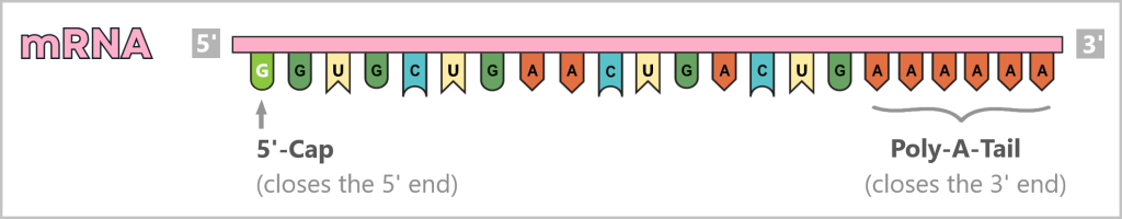
Primer binds: To let the reverse transcriptase know where to start, a primer is needed – a short DNA fragment that often binds specifically to the poly-A tail.
Reverse transcriptase gets to work: It attaches to the primer and reads the RNA bases (A, U, G, C) of the template. Then it adds the matching DNA bases (A, T, G, C) one by one – building a complementary DNA strand. The result is a hybrid molecule made of RNA and DNA (an RNA–cDNA hybrid).

Both the 5′ cap structure and the poly-A tail of the RNA do not appear in their original form in the resulting cDNA. The 5′ cap is typically ignored, while the poly-A tail is represented in a complementary form and may be partially shortened.
From single strand to double strand: This first DNA strand now serves as a template itself – a second strand is synthesized, resulting in double-stranded cDNA (ds cDNA). This form is stable and ready for PCR.

What does the whole process look like in action? This animation shows cDNA synthesis in fast-forward – explained simply and clearly.
4️⃣ What do you need for a PCR?
Before amplification can begin, a few ingredients and tools need to be ready:
a) DNA template: The starting material is the double-stranded cDNA that was produced from viral RNA in the previous step.
b) Nucleotides – the building blocks: Four different building blocks are needed to copy DNA: adenine (A), thymine (T), cytosine (C) and guanine (G). These will later be assembled by the polymerase into a new strand.
c) DNA polymerase – the master builder: This enzyme reads the DNA template and assembles the matching nucleotides into a new strand – precise and lightning-fast. In PCR, a heat-stable polymerase (e.g., Taq polymerase) is often used to withstand the high temperatures of the PCR cycles.
d) Primers – the guides: Primers are short DNA fragments (usually 18–24 bases long) that show the polymerase where to start copying. For PCR, you always need two: a forward primer and a reverse primer, which bind to opposite strands of the target DNA.

e) Buffer solution – the right environment: It ensures the polymerase is comfortable, providing a stable pH value, magnesium ions, and everything the enzyme needs for reliable function.
f) Thermocycler – the temperature carousel: A device that automatically runs the necessary temperature cycles. It heats, cools, and maintains precise temperatures – timed perfectly for the different PCR steps.

5️⃣ The process of the Polymerase Chain Reaction (PCR)
All the ingredients – DNA template (ds cDNA), nucleotides, DNA polymerase, primers, and buffer solution – are combined in a small reaction tube. This tube is then placed in the thermocycler, which automatically runs the typical PCR temperature cycles. Each cycle consists of three main steps:
Step 1 – Separation of DNA strands (Denaturation): The sample is heated to about 94–98 °C for around 20–30 seconds. This breaks the hydrogen bonds between the DNA bases – the double strand „melts” into two single strands. These single strands then serve as templates in the next step.

Step 2 – Primer binding (Annealing): The temperature is lowered to 50–65 °C. Now, the primers specifically bind to their respective single strands. They mark the starting point for DNA synthesis. The primers are designed to bind only to viral sequences – not to human RNA or DNA.

Step 3 – DNA synthesis (Amplification): At around 70 °C, the optimal temperature for the polymerase, the actual copying begins. The DNA polymerase binds to the primer, reads the single strand from 3′ to 5′, and synthesizes the new strand in the 5′ to 3′ direction. It assembles nucleotides following base-pairing rules: A pairs with T, and G pairs with C. This results in two new double-stranded DNA molecules.

This step is called amplification (from Latin amplificatio: enlargement), elongation (from Latin elongare: to lengthen), or polymerization (from Greek poly: many; meros: part).
6️⃣ Repeating the Cycles
The newly formed double-stranded DNA molecules immediately serve as templates for the next round. The steps – denaturation, primer annealing, and DNA synthesis – are repeated in cycles.
With each cycle, the amount of DNA doubles: 1 → 2 → 4 → 8 → 16 → 32 …
After just 25 – 40 cycles, billions of copies of the target DNA segment are produced.

📈 What is present at the end of RT-PCR:
A highly concentrated solution of specific DNA fragments – directly derived from the viral RNA. In the case of the influenza virus, it contains only those genome segments that were specifically targeted.
This DNA now serves as the basis for further analyses:
➤ to confirm the identity of the virus,
➤ to distinguish between different virus variants,
➤ or to quantify the viral load in the patient sample.
🎥 Tip: The video „What is PCR? Polymerase Chain Reaction” provides a clear summary of the process. Even though it focuses on human DNA, the core principle remains exactly the same.
b) Random Primed PCR
💡Note: If you’re not yet familiar with PCR, start by reading the section „PCR – Step by Step”. It clearly explains the basics and workflow. The following content builds on that foundation and focuses specifically on the unique aspects of Random Primed PCR.
Random Primed PCR is a special variant of PCR that is primarily used when a virus is unknown or its genome is highly variable.
In contrast to classical PCR, which uses specific primers to selectively amplify defined DNA segments, this method employs so-called random primers: short DNA sequences with randomly arranged bases that can bind at many positions along the target DNA (or cDNA) – regardless of its exact base sequence.
Advantage: Even unknown or highly mutated regions of the genome can be co-amplified using this method – a crucial benefit when preparing for sequencing, where the exact base sequence needs to be determined.
Examples of Random Primers:
Hexamer Primers  (6 bases long): AGCTGA, CTAGCT, …
Heptamer Primers (7 bases long): CCTGAGT, GATTACA, …
Nonamer Primers  (9 bases long): GCAGTTCGC, ATGGCCGTA, …

In practice, mixtures of all possible primer variants are usually used (e.g., 4⁶ = 4096 combinations for hexamers). This ensures that as many binding sites as possible in the genome are targeted.
Process of Random Primed PCR
Step 1 – Denaturation: The DNA (or cDNA) is heated to about 95 °C to separate the two strands. This creates single strands to which the primers can bind.
Step 2 – Primer Binding: The temperature is lowered so that the random primers can attach to many different sites on the DNA. Since the primers are random, they can bind to a variety of positions within the genome.
Note on genome size: Viruses have very different genome lengths – ranging from a few thousand to hundreds of thousands of base pairs. Random primers help to cover as much of the genome as possible.
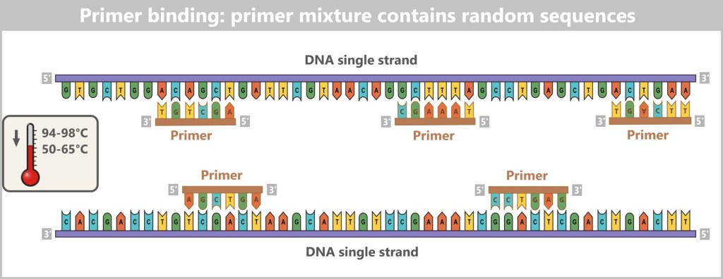
Step 3 – DNA synthesis: The DNA polymerase binds to the primers and starts synthesizing new DNA strands from there. It reads the template until it either reaches the end or encounters another primer. This acts like a stop signal – resulting mostly in shorter DNA fragments.
This is exactly what is intended: the polymerase generates many short, overlapping fragments that can later be used for genome reconstruction or targeted analyses.
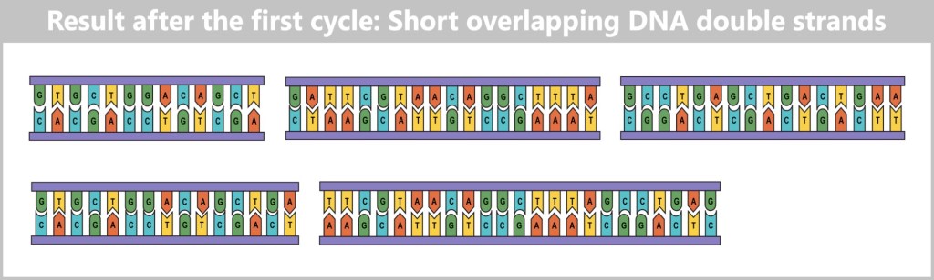
After the activity of the DNA polymerase, multiple short, overlapping double-stranded DNA fragments have formed from the single strands. These fragments are the result of the first cycle of the Random Primed PCR.
🔁 Cyclic Repetition
This process is repeated multiple times – just like in classic PCR – usually 20 to 40 cycles.
- The more cycles, the more DNA is produced.
- With increasing cycle number, the chance that primers „catch” each other rises → resulting in shorter fragments.
- However: Too many cycles can reduce diversity because some regions become overrepresented.
A balanced number of cycles and a well-optimized primer mix are crucial for the quality and representativeness of the final product.
📈 Result of the Random Primed PCR
In the end, a large number of short, overlapping DNA fragments are present – not complete strands, but a mosaic of fragments that can cover the entire viral genome.
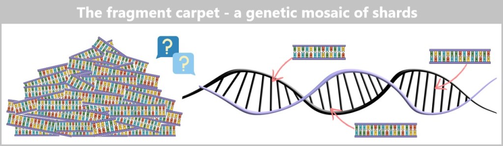
🧩 What happens to the DNA fragments?
Direct analysis of individual fragments
Often, it’s enough to sequence specific fragments to gain important information – e.g., for mutation analysis or virus typing.
Reconstruction of the entire genome
If the whole genome is to be analyzed (e.g., for discovering new viruses or for creating phylogenetic analyses), the fragments are read using sequencing technologies (more on this in the next chapter). Specialized software programs then piece together the overlapping fragments like a puzzle.
🧬 From Fragment to Complete Genome
Amplification using Random Primed PCR is just the first step – it ensures that enough genetic material is available for further analyses. However, simply multiplying the material is not enough to truly understand which virus you are dealing with.
Now it’s about determining the exact sequence of base pairs in the generated DNA fragments – in other words, their sequencing. Only through this sequencing can the genetic profile of the virus be decoded: mutations can be identified, viral strains distinguished, and even evolutionary family trees constructed.
In the following chapter, we therefore take a look at how sequencing works, which technologies are used for this – and how a complete viral genome is reconstructed from many small DNA snippets.
4.5.3. Sequencing
Sequencing is THE crucial step in decoding the genetic material of viruses. It determines the exact order of the bases in DNA (A, T, C, G) or RNA (A, U, C, G).
What’s the point?
A viral genome sequence is like the QR code of biology: Once scanned, you immediately know what you’re dealing with.
Identification of the virus:
🔹 Which virus is it exactly?
🔹 Is the virus already known or is it a new discovery?
🔹 Which virus family or genus does it belong to?
Detection of mutations:
🔹 Has the virus changed – and if so, how?
🔹 Have new variants or strains emerged?
🔹 What genetic differences exist compared to earlier versions?
Determination of diagnostic markers:
🔹 Are there stable (conserved) regions in the genome that are suitable for diagnostic tests?
🔹 Are there genes or proteins that are unique to this virus?
🔹 Can certain genes or proteins be specifically targeted – for example, for drug development?
Sequencing gives each virus a genetic fingerprint – unique, precise, and tamper-proof.
🧬 From Test Tube to High Technology
Decoding viral DNA used to be manual labor – today, it’s high-tech. Modern sequencers analyze millions of DNA fragments simultaneously – fast, automated, and with high precision.
Since the first manual procedures, technology has developed rapidly. Each new generation has made the view into the genome clearer, faster and more comprehensive.
The following overview shows how sequencing has evolved – and which technologies are available today:
| Generation | Description |
|---|---|
| First Generation: Sanger Sequencing | The old-timer: slow but precise. Ideal for short sections. |
| Second Generation: Next-Generation Sequencing (NGS) | The high-throughput powerhouse: sequences millions of DNA fragments simultaneously. |
| Third Generation: Real-Time Sequencing | The quantum leap – single molecule analysis in real time. |
| Emerging Technologies | Science fiction becomes reality. |

First Generation: Sanger Sequencing
Sanger sequencing, named after the British biochemist Frederick Sanger, marks a historic milestone in molecular biology. With this method, he was the first to successfully determine the exact sequence of DNA bases – a scientific breakthrough that earned him his second Nobel Prize in Chemistry in 1980.
Although more modern and automated methods are now available, Sanger sequencing is still considered the gold standard when it comes to the highest accuracy for short DNA segments. It is still widely used in many laboratories to validate results.
It is based on the principle of terminating DNA synthesis. During the copying process, special stop signals are incorporated, creating DNA fragments of varying lengths. These fragments are then sorted by size, allowing the sequence of building blocks to be read.
How the classic DNA analysis works
1️⃣ DNA Denaturation
First, the double-stranded DNA is heated. The high temperature breaks the hydrogen bonds between the base pairs, causing the double strand to separate into two single strands. These single strands then serve as templates for synthesizing new DNA.
2️⃣ Preparation of the reaction mixtures
Four separate reaction mixtures are prepared. Each contains:
➥ Single-stranded DNA: the template.
➥ Primer: a short sequence that provides the starting point for the polymerase.
➥ DNA polymerase: the enzyme that synthesizes new strands.
➥ dNTPs (deoxyNucleosideTriPhosphates): the „standard” DNA building blocks (A, T, C, G). They enable DNA strand extension because their 3′ hydroxyl group can bond with the next building block.
➥ ddNTPs (didesoxyNukleosidTriPhosphate): these „modified” DNA building blocks lack a hydroxyl group, so no further nucleotides can be attached after them. When a ddNTP is incorporated during synthesis, the DNA strand elongation stops exactly at that point. Each of the four ddNTP types (A, T, C, G) is additionally labeled with its own fluorescent dye.
The ratio of dNTPs to ddNTPs is carefully adjusted to generate a wide range of DNA fragments of varying lengths.
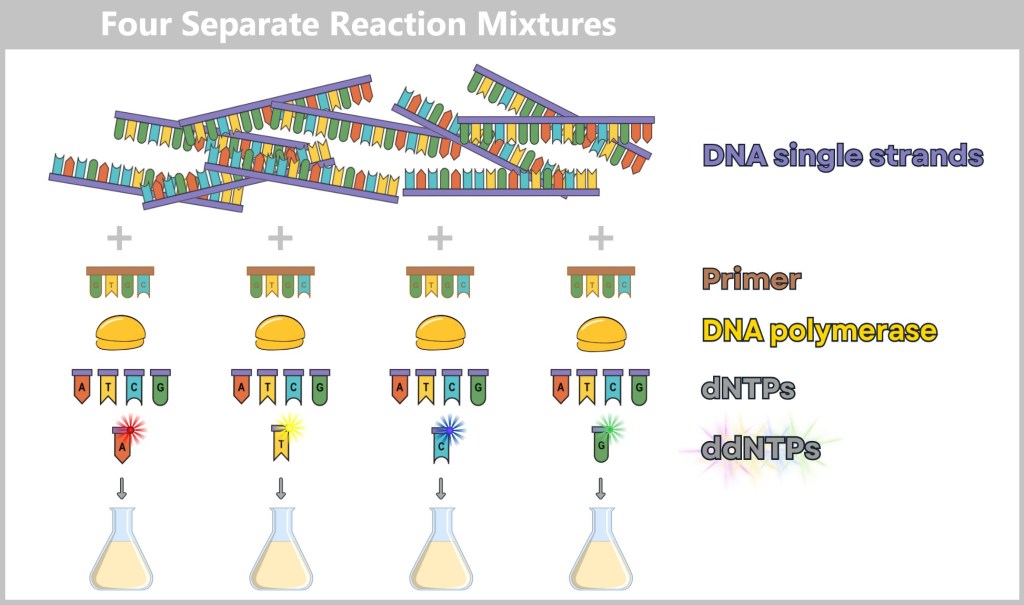
3️⃣ DNA Synthesis with Random Termination
DNA synthesis – briefly explained: DNA polymerase is nature’s most efficient copier. It scans a DNA strand as a template and builds a matching complementary strand step by step – always following the base-pairing rules: A pairs only with T, and C only with G. The result is a perfect mirror copy.
DNA synthesis takes place simultaneously in the four separate reaction mixtures – one for each of the four bases (A, T, C, G).
Here’s what happens in each mixture: The DNA polymerase binds to the primer and gets to work.
How to find the right primer?
Primers are absolutely essential for the successful use of the Sanger method. But how do you find the primer sequence when the genome of a virus is completely unknown?
When Frederick Sanger developed his method in 1977, some information about the genome structure of small viruses like the bacteriophage Phi-X174 was already known. Researchers had discovered that certain enzymes – called restriction enzymes – cut DNA at very specific sites. These cutting sites were known and could be used deliberately:
Near these cutting sites, there was often a short piece of known DNA sequence – just enough to design a suitable primer. This way, researchers artificially created a defined starting point for the sequencing process.
Today, it’s easier. Science has advanced significantly, and most viruses are already well studied. For new or little-known viruses, the following approach is used:
Comparison with known viruses: Often, a new virus is genetically similar to already known viruses. Scientists use these similarities to predict possible primer sites.
Experimental approaches: When little is known, enzymes cut the viral DNA into smaller fragments. Researchers then analyze these fragments to identify suitable starting points for primers.
It reads the single-stranded DNA template and inserts matching building blocks (dNTPs) to synthesize a new DNA strand.
Normally, a „regular” dNTPs is incorporated – allowing the DNA chain to continue growing. Occasionally, however, a modified ddNTP is incorporated – and synthesis stops immediately at that point. This happens because ddNTPs lack a small chemical group (the hydroxyl group) that’s essential for adding the next nucleotide.
This results in many DNA fragments of different lengths – each one ending precisely at the point where a ddNTP was randomly incorporated. And each fragment carries a fluorescent dye at its end, indicating which type of base (A, T, C, or G) the fragment terminates with.

Each reaction mixture contains one modified nucleotide (ddATP, ddTTP, ddCTP, or ddGTP). When this modified nucleotide is incorporated during DNA synthesis, the process stops exactly at that position, because the modified building block does not allow further extension of the DNA chain. In the ddATP mixture, synthesis stops when adenine (A) is incorporated. In the ddTTP mixture, the chain is terminated when thymine (T) is added. Similarly, ddCTP and ddGTP cause termination at cytosine (C) and guanine (G), respectively. This method generates DNA fragments of varying lengths, each ending with the specific stop nucleotide. The goal is to produce all theoretically possible sequence fragments.
4️⃣ Denaturation of the Fragments
The resulting double-stranded DNA fragments are heated again so that they separate into single strands. This step is necessary to allow individual analysis of each fragment. What remains is single-stranded DNA – ready for the next step.
5️⃣ Analysis
Now it’s time for analysis: The fragments are separated by size using gel electrophoresis. For this, the four reaction mixtures are loaded into separate wells of a gel.
The gel acts like a fine mesh or sponge:
- Short fragments move through faster.
- Longer fragments move more slowly.
Each strand ends with a color-labeled ddNTP – depending on the base (A, T, C, or G), a different color lights up. These colors are detected by a laser and recorded automatically.
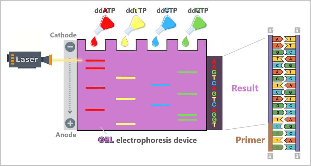
In the reaction tubes are DNA fragments of different lengths, each ending with the same terminating nucleotide (depending on the mixture: adenine, thymine, guanine, or cytosine). The reaction mixtures are loaded onto the gel. Under the influence of an electric field, the negatively charged DNA fragments migrate from the cathode (−) to the anode (+). The size of the fragments determines their migration speed through the gel. Smaller DNA fragments move faster through the gel pores and thus reach the anode first, while larger fragments progress more slowly. By reading the fluorescent signals, the base sequence of the DNA can be determined.
How do you read the sequence from this?
The order of the fragments in the gel corresponds to the order of the bases in the original DNA strand.
- The shortest fragment shows the first base.
- The next longer fragment shows the second base,
- … and so on, until the entire sequence is decoded.
Since each new fragment is complementary to the original strand, the base sequence of the original DNA strand can be directly deduced from the analysis.
🎥 Tip: You’ll find a very clear explanation in the video „Sanger Sequencing / Chain Termination Method”.
Where is Sanger sequencing used?
This method is especially well suited for:
- Short DNA fragments
- Confirmation and validation of results from other methods
- Individual case analyses, e.g., in medical diagnostics
Some methods don’t get old – they become classic.
Limitations of the method
As precise as Sanger sequencing is, it quickly reaches its limits with large or complex genomes. The method is labor-intensive, time-consuming, and expensive, especially when many samples or extensive datasets need to be analyzed. For this reason, it has been replaced in many areas by modern high-throughput techniques – above all, by Next-Generation Sequencing (NGS) technologies.
Second Generation: Next-Generation Sequencing (NGS)
Next-Generation Sequencing (NGS) is a modern method for decoding DNA and RNA sequences – and has fundamentally transformed genetic research since the early 21st century. Compared to classical Sanger sequencing, NGS is faster, more cost-effective, and can process significantly larger volumes of data in a shorter amount of time.
The key difference: While the Sanger method sequences only a single DNA fragment at a time, NGS can read millions of fragments simultaneously. To achieve this, the genetic material is first broken down into small pieces and tagged with special markers. These fragments are then fixed onto a special surface and extended step by step using fluorescently labeled nucleotides – each newly incorporated base is immediately detected and recorded.
Thanks to this parallel processing, a high-resolution dataset is generated within a short time – ideal for analyzing entire genomes, RNA profiles, or large sample volumes. This is precisely why NGS is now a key technology in research, diagnostics, and biotechnology.
A Closer Look at Illumina Sequencing
Illumina sequencing is one of the most widely used technologies in the field of Next-Generation Sequencing (NGS). It is based on the principle of „sequencing by synthesis” and enables the simultaneous reading of millions of DNA fragments. Here’s a step-by-step explanation:
Step 1: DNA Preparation = Library Construction
Step 2: Cluster Generation on a Flow Cell
Step 3: Sequencing by Synthesis
Step 1: DNA Preparation = Library Construction
Before sequencing, the DNA must be converted into a format compatible with the Illumina platform. This process is known as library construction and includes the following sub-steps:
1a) Fragmentation
The DNA is fragmented into smaller pieces either mechanically or enzymatically (typically targeting a size range of around 150–500 base pairs). This process produces DNA fragments of slightly varying lengths, which are often further standardized using a size selection step.
To illustrate this step, we will consider three DNA fragments with slightly different lengths in our example.
1b) Adapter Ligation
Specific adapter sequences (P5 and P7 adapters) are ligated to both ends of the DNA fragments. These adapters serve several important functions:
Binding Sites for the Flow Cell: The adapters contain special DNA sequences that function like a key fitting into a lock. This allows the DNA fragments to adhere to a surface later, which is important for sequencing.
Primer Binding Sites: The adapters contain regions where sequencing primers can bind. These primers are later used to gradually synthesize the DNA strands during the sequencing process.
Indexes (optional): If multiple samples are sequenced simultaneously, index sequences allow the fragments to be assigned to their respective samples.
For clarity, we omit the depiction of indexes in our example.
1c) PCR Amplification
To ensure that enough DNA is available for sequencing, the adapter-ligated DNA fragments are amplified using the polymerase chain reaction (PCR).

The following close-up shows a detailed view of a fragmented double-stranded DNA molecule equipped with the two adapters.

Each DNA fragment (DNA insert) receives two adapter sequences:
The P5 adapter consists of the P5 adapter sequence, which enables binding to the flow cell, and the primer binding site Rd1SP (Read 1 Sequencing Primer) for initiating DNA synthesis. Similarly, the P7 adapter contains the P7 adapter sequence for flow cell binding as well as the primer binding site Rd2SP (Read 2 Sequencing Primer) to initiate DNA synthesis.
Important note: The upper and lower single DNA strands each carry P5 and P7 adapters. However, the adapters on the lower strand are not identical but complementary to the adapters on the upper strand.
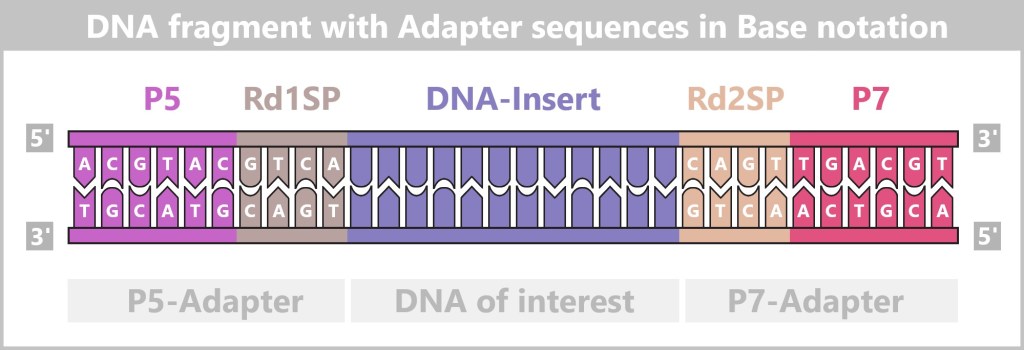
This representation is highly simplified. In practice, Illumina adapter sequences are much longer, typically consisting of 60–120 base pairs (see here). The DNA insert is also shortened for better illustration – in reality, DNA fragments usually range from 100 to 500 base pairs in length.
Step 2: Cluster Generation on a Flow Cell
Before the DNA can be sequenced, it must be fixed and amplified on a solid surface. This takes place on a flow cell, a special glass plate equipped with millions of tiny DNA binding sites.
The goal of this step is to generate numerous copies of each DNA fragment on the surface to amplify the signals during sequencing. For this purpose, the flow cell is coated with special oligonucleotides (DNA molecules) that are complementary to the adapter sequences of the DNA fragments. There are two types of these oligonucleotides:
- P5 oligonucleotides (ACGTAC), which bind to the P5 adapters (TGCATG) of the DNA fragments.
- P7 oligonucleotides (ACGTCA), which interact with the P7 adapters (TGCAGT) of the DNA.
You can imagine the surface of the flow cell like a dense Velcro strip: The DNA fragments stick to it with their adapter sequences, similar to tiny hooks catching onto the Velcro fabric.

2a) DNA fragments bind to the flow cell surface
At the beginning of this step, a solution containing single-stranded DNA fragments with adapter sequences is flowed onto the flow cell. These fragments were previously separated into single strands by denaturation, allowing them to move freely in the solution.
As the DNA fragments flow through the flow cell, their adapters bind to the complementary oligonucleotides on the flow cell surface through base pairing, as shown in the illustration below.

P5 adapter of a single-stranded DNA binds to the P5 oligonucleotide on the flow cell:
Flowcell — P5-Oligo  ACGTAC
         — (3')      TGCATG-CAGT-[Insert]-GTCA-ACTGCA (5')
P7 adapter of a single-stranded DNA binds to the P7 oligonucleotide on the flow cell:
Flowcell — P7-Oligo  ACGTCA
         — (3')      TGCAGT-TGAC-[Insert]-ACTG-CATGCA (5')
2b) First synthesis
Primer binding and DNA synthesis
After the DNA fragments have bound to the flow cell, the first DNA synthesis begins. Specific primers bind to the adapter sequences of the bound strands:
- Primer GTCA binds to the P5 adapter of the bound single strand.
- Primer ACTG binds to the P7 adapter of the bound single strand.
The DNA polymerase, which can only work in the 5′ → 3′ direction, then synthesizes a new strand complementary to the already bound single strand.

After synthesis, the bound DNA fragments exist as double strands.
Flowcell (P5-Oligo) — (5') ACGTAC-GTCA-[Insert]-CAGT-TGACGT (3')
                    — (3') TGCATG-CAGT-[Insert]-GTCA-ACTGCA (5')
Flowcell (P7-Oligo) — (5') ACGTCA-ACTG-[Insert]-TGAC-GTACGT (3')
                    — (3') TGCAGT-TGAC-[Insert]-ACTG-CATGCA (5')
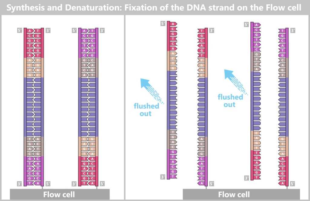
Separation of the double strand
After the new DNA strand has been synthesized, the double strand is separated by denaturation (see the figure above):
❌ The original strand is no longer attached to the flow cell after denaturation and is washed away.
✅ The newly synthesized strand remains firmly attached to the flow cell via its 5′ end, while the 3′ end remains free.
Now the DNA fragments are bound to the flow cell as complementary single strands (forward and reverse strands).
However, direct sequencing at this stage would not be possible, as the fluorescence signals would still be too weak to be reliably detected. This is why bridge amplification follows next.
2c) Bridge Amplification
To generate a sufficiently strong fluorescence signal for DNA sequencing, the individual DNA strands must be amplified. This is achieved through bridge amplification – a cyclic process in which the DNA strands bind to the flowcell surface, are copied, and then separated again.
Hybridization of the Second Adapter
Bridge amplification begins with the bound single-stranded DNA bending over and hybridizing its free 3′-end to a nearby complementary oligonucleotide (5′) on the flowcell surface. This process is known as strand folding. It creates a loop-like structure – a „bridge” – that connects the adapter on the DNA strand to the matching surface oligonucleotide.
DNA Synthesis
Once the DNA strands are hybridized, primers (e.g., ACTG, GTCA) and DNA polymerase are added. The primers bind specifically to the adapter sequences. DNA polymerase then synthesizes new complementary strands in the 5′ → 3′ direction. After synthesis, the DNA is once again present as a double-strand.
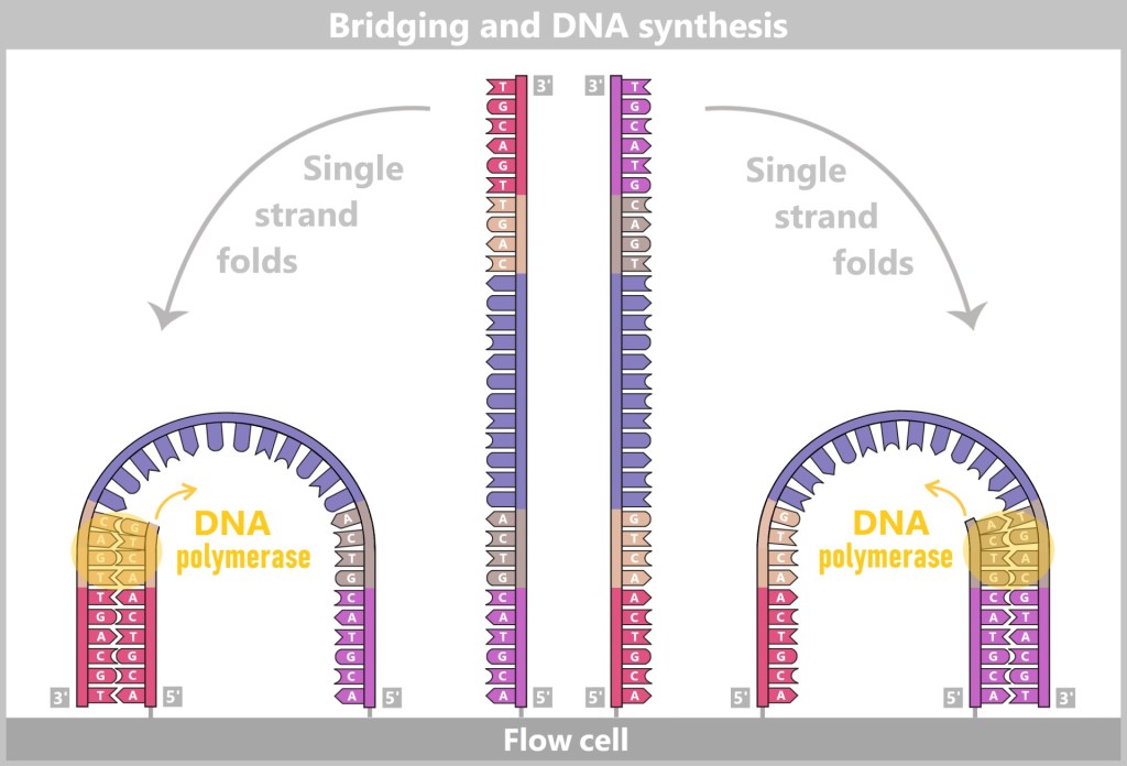
The bound single DNA strands fold over and hybridize with a complementary oligonucleotide on the flowcell, forming a bridge-like structure. A primer then binds to the 3′ ends of the strands, and DNA polymerase synthesizes the complementary strands in the 5′ → 3′ direction.
Denaturation – Strand Separation
Heat or chemical treatment is used to separate the newly formed double-stranded DNA into single strands again. At this point, there are four single-stranded DNA fragments on the flowcell:
|| the original two single strands (forward strand & reverse strand), and
|| the newly synthesized complementary strands (forward strand & reverse strand).
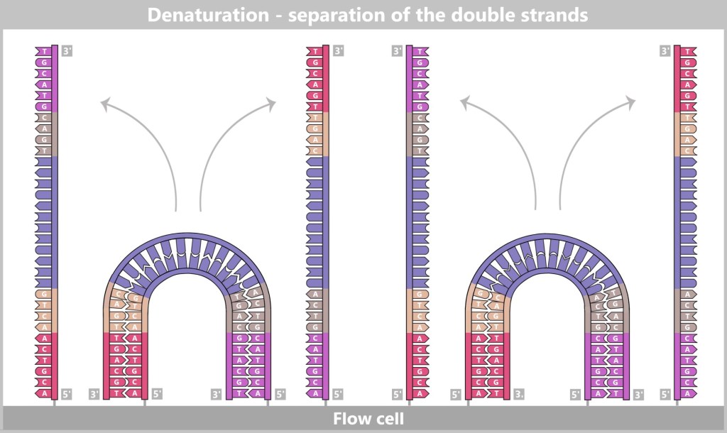
After denaturation, the bridge double strands are separated, so that on the flow cell there are now two single strands (forward and reverse) visible. These single strands remain attached to the flow cell and are ready for further amplification.
Repeat amplification
This cycle repeats: The single strands fold again, hybridize once more with the oligonucleotides, and are duplicated through DNA synthesis.

After multiple cycles, millions of identical copies of each original DNA fragment – called clusters – are formed on the flow cell.
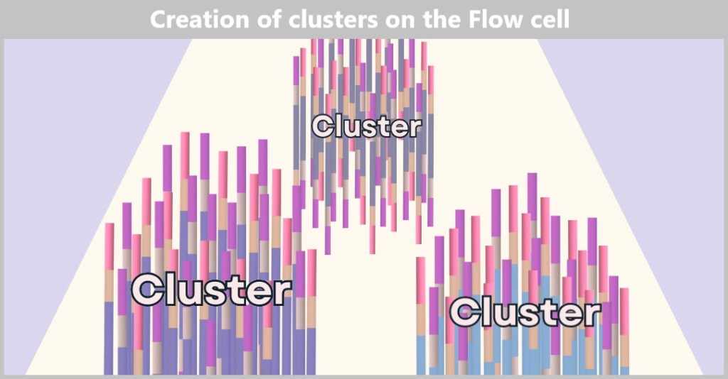
Each cluster consists of numerous copies of a single DNA fragment. In this illustration, only three clusters are shown as examples, based on our example of three DNA fragments. In reality, however, millions to billions of such clusters are present on a flow cell to enable high sequencing capacity.
Formation of the final clusters
At the start of our example, three DNA fragments are present. After several amplification cycles, countless clusters form for each of these fragments, each consisting solely of copies of their respective DNA fragment.
Each cluster now consists of two types of strands:
🔹 Forward strands (5′ → 3′, bound to P7)
🔹 Reverse strands (3′ → 5′, bound to P5)
💡Note: Forward and reverse strands within the clusters are not aligned antiparallel to each other! Instead, the 3′ ends of both strands point upwards.
Removal of the reverse strands
For the sequencing to proceed correctly, all DNA strands within a cluster must be oriented in the same direction. Only the forward strands are needed for the actual analysis. Therefore, a targeted purification step follows:
🔹 All reverse strands (bound to P5) are detached and washed away.
🔹 At the same time, the free ends of the P5 oligos are chemically blocked to prevent reattachment.
Now, only forward strands remain on the flowcell. The clusters are fully formed, and the DNA libraries are ready for sequencing.

Left: A final cluster with forward (P7-bound) and reverse strands (P5-bound). Right: The reverse strands have been selectively cleaved and washed away, leaving only the forward strands. This orientation is necessary to carry out sequencing correctly.
Step 3: Sequencing by Synthesis
At this point, individual clonal clusters (originating from the initial three DNA fragments) are distributed across the entire surface of the flow cell. Each cluster consists of numerous identical DNA copies – comparable to a small island of identical trees. Now, the actual sequencing can begin.
To start the sequencing, primers, DNA polymerases, and modified nucleotides are applied to the flow cell.
The modified nucleotides have three special properties:
① Termination of synthesis
They carry a chemical modification on the hydroxyl group that prevents the addition of another nucleotide to the growing DNA strand. As a result, DNA synthesis stops immediately after the incorporation of each individual nucleotide.
② Reversibility of the blockage
This modification can subsequently be chemically removed, allowing DNA synthesis to continue. This enables sequencing to proceed step-by-step, one nucleotide at a time.
③ Fluorescent labeling
Each of the four bases (A, T, C, G) is tagged with a specific fluorescent dye.
Because of these properties, these nucleotides are called reversible terminator nucleotides (RT-dNTPs).
Sequencing Process
➥ The sequencing primers hybridize to the forward strands of the DNA library.
➥ DNA polymerase binds to the primer and begins synthesis. However, due to the modified nucleotides, it can add only one nucleotide per cycle.
➥ After each incorporation, the flow cell is photographed by a high-resolution camera. The fluorescent label indicates which nucleotide was added. A computer analyzes the fluorescence signals and assigns them to the corresponding bases.
➥ Then, excess nucleotides are washed away, and the blocking group on the incorporated nucleotide is chemically removed.
➥ The cycle starts again, repeating until the entire DNA fragment has been sequenced.

Primer, DNA polymerase (DNAP), and modified nucleotides (RT-dNTPs) are applied to the flowcell. The RT-dNTPs are fluorescently labeled (each base has its own color) and carry a reversible block at the 3’-hydroxyl group. This causes DNA synthesis to pause temporarily after each base incorporation.
As soon as an RT-dNTP is incorporated, a laser excites the fluorescent dye, causing it to emit light. A camera captures this signal and determines which base was added. Then, the fluorescent label along with the blocking group is chemically removed, allowing DNA synthesis to continue in the next cycle. This process is repeated in every cycle: one base is added, the signal is recorded, and the block is removed. The sequencing proceeds over a set number of cycles, reading a limited number of bases (e.g., 150 base pairs in 150-base reads).

During sequencing, a camera captures the fluorescence signals of the incorporated nucleotides in each cycle. Each cluster emits a specific color signal that corresponds to the incorporated base. Over the course of multiple cycles, this generates a unique sequence for each cluster. A computer analyzes the color information from the individual images and assigns it to the corresponding DNA sequence. In this way, the precise base sequence of the „DNA of interest” is reconstructed from the measured fluorescence signals.
Double-check for DNA: Paired-End Sequencing
Paired-end sequencing is a method commonly used on many Illumina platforms to improve the accuracy and reliability of sequencing results. In this approach, each DNA fragment is read from both ends – resulting in two reads per fragment: Read 1 (forward) and Read 2 (reverse).
After the initial sequencing of the forward strand (Read 1), a second round of bridge amplification is performed to regenerate the original DNA strands. The previously sequenced strands are then removed, and sequencing of the reverse strand (Read 2) begins.
Since both reads originate from the same DNA fragment, they can be computationally merged. This facilitates sequence assembly, enhances error detection, and improves the readability of repetitive or complex regions within the DNA sequence.
Paired-end sequencing is particularly well suited for long, nested, or challenging DNA regions – providing more precise and reliable results.
Result of Illumina Sequencing
At the end of Illumina sequencing, a vast amount of short DNA segments – known as reads – is obtained. Each of these reads originates from a small fragment of the original genetic material and has been amplified and read millions of times.
To reconstruct a complete picture from these reads, specialized software is used to assemble them on a computer:
🔹 If a known reference DNA is available, the reads are aligned like puzzle pieces to the existing sequence pattern.
🔹 If no template is available, the reads must be assembled piece by piece based on overlapping regions.
This step-by-step assembly of countless short sequences gradually creates a complete picture of the original DNA material. The result is a precisely analyzed gene sequence that not only reveals the genetic structure but also provides insights into mutations or variants.
🎥 Tip: You can find a clear explanation in the video „Illumina Sequencing Technology”.
Applications
Illumina sequencing is known for its accuracy and reliability. Its applications include:
Genomics: Decoding the DNA of humans, animals, and plants
Medicine: Investigating genetic diseases and developing personalized therapies
Microbiology: Analyzing bacteria and viruses
Environmental research: Studying DNA in soil or water samples
And what comes next?
Illumina technology has revolutionized genetic analysis – but it also has its limits: the preparation is complex, data analysis is computationally intensive, and very long DNA segments can only be read in small fragments.
That’s why development continues. New third-generation sequencing technologies rely on entirely different principles – enabling, for the first time, the direct reading of extremely long DNA strands, often even in real time.
Time to take a look at the next generation of sequencing.
Third Generation: Real-Time Sequencing
With the third generation of sequencing technologies, a fundamental shift is beginning in genomic research. Instead of relying on fragmented or chemically modified DNA as before, these methods allow for the direct reading of genetic information – in real time, without complex preparation, and with new analytical possibilities.
Two key methods of this generation are:
- Single Molecule Real-Time (SMRT) Sequencing – monitors DNA synthesis in real time by detecting light pulses emitted as individual bases are incorporated.
- Nanopore Sequencing – threads DNA strands through tiny nanopores and measures changes in electrical current to identify the bases.
Why Nanopore Sequencing Is a Game Changer
Nanopore technology opens up entirely new perspectives in genomic research – thanks to its flexibility, speed, and independence from labor-intensive preparation steps:
✅ Real-time sequencing: Unlike traditional methods that require DNA to be amplified or chemically modified first, nanopore technology reads genetic material directly.
✅ Long read lengths: Instead of short fragments, extremely long DNA strands can be read – often spanning hundreds of thousands of base pairs in a single run. This greatly simplifies the analysis of complex genomes and structural variants.
✅ Versatility: In addition to DNA, RNA can also be analyzed directly – without the intermediate step of converting it into complementary DNA (cDNA). This makes the technology especially valuable for studies of gene expression and virus research.
✅ Portable and cost-effective: Devices like the MinION are barely larger than a USB stick and enable sequencing outside the lab – such as in clinics, in the rainforest, or directly at a crime scene.
With these features, nanopore sequencing opens up entirely new fields of application – from basic research and diagnostics to environmental and biodiversity analysis.
That’s reason enough to take a closer look at this technology.
For a first impression and a brief overview, the following video is a great starting point.
Nanopore Sequencing – Step by Step
Today, when people talk about nanopore sequencing, they almost always mean Oxford Nanopore Technology (ONT). While there are theoretically other nanopore-based approaches, ONT is currently the only one in practical use. Since its general market launch in 2015, it has revolutionized sequencing.
What makes this method special? It reads DNA or RNA directly and in real time – without prior chemical modifications or amplification reactions. Nanopore technology functions like a tiny high-performance laboratory that decodes genetic information with precision.
How does it work?
ONT sequencing is based on the interaction of three key components:
➤ Nanopores – act as tiny molecular „readers”. When a DNA or RNA strand passes through a nanopore, it generates characteristic electrical signals – essentially a molecular „fingerprint”.
➤ Membrane – serves as a filter and barrier. It ensures that only ions and nucleic acids pass through the nanopores, while unwanted molecules are kept out. This results in clean, precise measurements.
➤ Chip – is the core of the system. It holds the membrane with the nanopores and detects the electrical signals generated as the DNA passes through.
The chip has two chambers:
- Upper chamber (cis): This is where the DNA sample is introduced.
- Lower chamber (trans): This is where the DNA ends up after passing through the nanopores.
Both chambers are filled with an ion-containing solution that conducts electrical current. The membrane separates the chambers so that no current can flow – except at the points where the nanopores are embedded. These pores are the only „tunnels” through which ions and nucleic acids can pass.
As soon as a DNA or RNA strand slides through a nanopore, the electrical current changes. These subtle variations are detected and translated into genetic code – in real time: directly, quickly, and accurately.
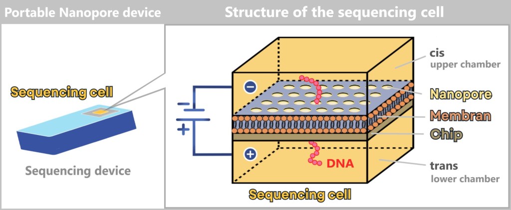
On the left is a portable nanopore sequencing device. In practice, it is slightly larger than a USB stick. An arrow points to the replaceable sequencing cell. The enlarged illustration on the right shows the schematic structure of the sequencing cell.
Precision at the Nanoscale
Chip microstructure
The chip is manufactured using highly precise fabrication techniques such as photolithography or etching processes. This creates tiny channels, called wells, that range from just a few nanometers to micrometers in size. In addition to these structural components, the chip also contains the electrochemical sensing device that detects the ion flow as DNA or RNA passes through the nanopore.
Self-assembly of the lipid membrane
This membrane consists of lipids (fat molecules) and is electrically insulating. This means that it does not conduct electricity itself. The membrane is initially applied onto the chip without nanopores. It is not mechanically stretched onto the chip, but is formed by self-organisation over the openings.
How does it work?
A solution containing lipid molecules is applied to the chip. These molecules have:
🔹 a hydrophobic (water-repelling) part, and
🔹 a hydrophilic (water-attracting) part.
Because of these properties, they spontaneously organize into a stable bilayer. The wells in the chip are designed so that the lipid membrane is stabilized precisely above them.
Self-assembly of the nanopores
Nanopores are usually made from proteins derived from bacteria or yeast cells. In nature, these pores serve as transport channels for molecules across cell membranes. However, in nanopore technology, they are used as highly sensitive sensors for DNA or RNA molecules.
The integration of the nanopores takes place after the membrane is formed. Thanks to a natural process called self-assembly, they insert themselves into the membrane spontaneously!
How does it work?
- The nanopores are added in a solution.
- They automatically „find” the wells, since they can only embed themselves in the membrane where an opening exists.
- There, they penetrate the membrane and form stable channels.
The wells are precisely defined areas where the membrane is accessible – and it is exactly there that the nanopores can integrate selectively.
Why is this important?
The correct positioning of the nanopores over the wells is crucial because:
- The wells are connected to electrodes that measure the ion flow. If a nanopore is not exactly positioned over a well, there is no measurable current – making the nanopore nonfunctional.
- DNA is pulled through the nanopores from the cis to the trans chamber, and this only works if the nanopores are embedded in the membrane directly above the wells.
The path of the DNA through the nanopore
After exploring the structure of the sequencing cell and the basic principle of Oxford Nanopore technology, we now turn to the actual sequencing process.
1️⃣ Preparation of the DNA/RNA sample
Before the actual sequencing begins, the nucleic acid (DNA or RNA) must be prepared.
➥ Extraction: The DNA or RNA is isolated from the sample (e.g., blood, saliva, cell culture, environmental samples). This is done using standardized extraction methods (see Chapter „4.5.1. Nucleic Acid Extraction” for details).
➥ Fragmentation (optional): Nanopore sequencing can read very long DNA or RNA molecules. If the DNA is too long or needs to be tailored for specific applications, it can be mechanically or enzymatically cut into fragments.
➥ Adapter ligation: Since the nanopores can only process DNA or RNA with special ends, adapters are attached to the ends of the molecules. These adapters contain:
- Motor proteins that control the movement of the DNA through the nanopore
- Barcode sequences (if multiple samples are to be sequenced simultaneously)

To enable the motor protein to bind to the DNA, special adapters are first attached to the DNA ends. These adapters ensure that the motor protein binds specifically at one end of the DNA. For clarity, the illustration shows only the binding of the motor protein, while the adapters themselves are not depicted. Typically, only one motor protein binds per DNA molecule, as the adapters are designed to favor binding at one preferred end.
Where does the motor protein come from?
The motor protein used in Oxford Nanopore sequencing is a naturally occurring enzyme derived from bacteria. It is a modified version of a protein originally found in organisms such as E. coli or other microorganisms. In nature, these proteins are responsible for unwinding and transporting DNA – a capability that nanopore technology harnesses for sequencing.
If RNA is to be sequenced, an optional reverse transcription step can be performed to convert RNA into DNA. However, ONT technology is capable of sequencing both RNA and DNA directly. Direct RNA sequencing can provide specific information about RNA modifications.
2️⃣ Applying an electrical voltage
Both chambers of the sequencing cell contain charged particles (ions). Once a voltage is applied between the upper (cis) and lower (trans) chambers, ions begin to flow through the nanopores. This creates a measurable electrical current. As long as no DNA is present in the pore, the ion flow remains constant, and a stable current is detected.
3️⃣ The DNA is added to the sequencing cell
The prepared DNA sample, with motor proteins already attached, is pipetted into the cis chamber (the upper chamber of the sequencing cell). Through diffusion or gentle mixing, the DNA disperses in the solution and reaches the vicinity of the membrane where the nanopores are embedded.
4️⃣ Docking onto the nanopore
The motor protein bound to the DNA guides the molecule to the nanopore and docks specifically onto it. Once the connection is established, the motor protein initiates its helicase activity: it unwinds the double-stranded DNA (dsDNA) into two single strands. One of these strands is captured by the nanopore and pulled through it. This process takes place directly at the pore and ensures that the DNA is transported precisely and evenly through the nanopore.

The sequencing cell consists of two chambers: the cis chamber (top) and the trans chamber (bottom), separated by a membrane with embedded nanopores. On the left, a DNA molecule has docked onto a nanopore with the help of a motor protein. On the right, an empty nanopore is shown, through which a constant ion current flows. The applied voltage between the negative electrode (cis) and the positive electrode (trans) drives the ion flow. The ion current is measured in the well (a small channel in the chip), as illustrated in the current/time diagram. As long as no DNA passes through the pore, the current remains constant.
5️⃣ The DNA passes through the nanopore – the signal is generated
DNA carries an electrical charge due to its negatively charged phosphate backbone. The applied voltage between the cis chamber (negatively charged) and the trans chamber (positively charged) causes the DNA to be pulled through the nanopore.
The motor protein plays a crucial role in this process:
➤ It controls the movement of the DNA through the pore – slowly, evenly, and steadily.
➤ This ensures a clearly readable signal for reliable signal detection.
For context: Naturally, DNA would shoot through the nanopore at a speed of millions of bases per second. The motor protein slows this down to about 450 bases per second (depending on the device and settings). This slowdown is what makes sequencing with this technology possible at all.
As the DNA passes through the pore, it influences the ion flow – because each base (A, T, G, C) has a unique size and chemical structure. These differences alter the ion current in specific ways. These current changes are measured by an electrode located directly beneath the nanopore. Each well (the tiny tunnels in the chip where the nanopores sit) has a dedicated electrode that acts as the sensor. This setup allows the software to precisely assign signals to a specific nanopore – an essential requirement for accurately reconstructing the DNA sequence.

1) A motor protein pulls the DNA steadily through the pore. The negatively charged DNA moves from the cis side to the trans side due to the applied voltage. During this process, the individual bases (A, T, G, C) affect the ion current in specific ways.
2) A graph displays the changes in the measured current over time. Each base combination produces a characteristic signal that is decoded by algorithms.
3) A computer analyzes the electrical signals and determines the sequence of the bases from them.
6️⃣ The electrical signal is recorded
As the DNA is pulled through the nanopore, about 10–15 bases are inside the pore at the same time. Each of these bases influences the ion current differently – so the signal is a composite of the effects of multiple bases.
But how can individual bases still be distinguished?
This works thanks to a clever algorithm:
- The motor protein moves the DNA step-by-step – roughly one base at a time.
- The measured current changes in characteristic ways depending on the sequence of bases.
- Specialized software (basecalling) uses machine learning to decode the exact sequence from the overlapping signals.
- The model „untangles” the overlapping information and assigns it to the correct base at the precise position.
In this way, the complete DNA sequence gradually emerges from the electrical signals.
Result of nanopore sequencing
In the end, Oxford Nanopore technology provides the complete sequence of bases in the analyzed DNA or RNA sample. This sequence contains detailed information about the genetic composition, the length of the molecules, as well as possible features such as mutations or structural variations.
🚀 Real-time data – a genuine speed advantage
The entire process happens live. As the DNA or RNA passes through the pore, the sequence of bases is captured and analyzed immediately.
For comparison:
- Traditional Sanger sequencing takes several hours or even days to complete an analysis.
- Illumina sequencing typically provides results within a few hours to several days, depending on the length, complexity, and scale of the sample – smaller projects often finish in a few hours, while larger analyses may take several days.
- Oxford Nanopore Technology (ONT), on the other hand, delivers initial results within minutes.
The generated sequencing data are processed and stored in parallel. They are immediately available for further analysis.
Looking ahead: Sequencing 4.0 – what’s next?
While the third generation is still being celebrated, researchers are already working on the fast lane. Emerging new technologies promise even more: greater speed, higher accuracy, and even more versatile applications.
In the next chapter, we’ll take a brief glimpse into the future of sequencing.
Emerging Technologies: The Future of Sequencing
Nanopore sequencing (ONT) has already revolutionized sequencing, but there are promising approaches in the tech pipeline that could further advance this method.
Transistor instead of pore
An exciting example is FENT technology (Field-Effect Nanopore Transistor), which analyzes DNA and other biopolymers using a novel transistor-based structure that operates with extreme speed and precision. This technology could enable even more precise, faster, and more cost-effective analysis of DNA and other biopolymers.
The „FENT Nanopore Transistor Explainer Video” offers a fascinating insight into this innovation.
Whether and when this technology will become relevant for virus diagnostics remains to be seen – but it impressively demonstrates how sequencing technologies continue to evolve.
The next big thing in genetics
Besides FENT, methods like In Situ Sequencing (ISS), which makes gene expression visible directly within tissues, could also play an important role in the future – such as investigating viral activity within cells.
The future of sequencing?
It’s going to blow us away – literally! –
and we’re right there live to witness it!
4.6. Bioinformatic Analysis
The raw sequencing data is simply a long string of bases, such as „AGCUACGUA…” in the case of an RNA sequence. Sequencing is like spelling – it’s only through bioinformatics that the story behind it is told, „translating” the data into meaningful information. From this jumble of letters (AGCUACGUA…), a profile is created: What virus is it? What can it do? And how dangerous is it?
Warum Rohdaten chaotisch sind
💨 Technical glitches: Like a blurry photo – some parts of the sequence are missing or fuzzy („noise”).
❓ Mystery bases („N”): Positions where even the machine gives up: „Could be A, C, or U – no idea!”
🦠 Mutant flatshare: RNA viruses like influenza exist as communities of variants (mutation clouds). Sequencing blends them all together – like a smoothie made from 100 different fruits.
What Bioinformaticians Do
They clean, sort, and piece together the data – until it becomes clear:
- Who’s here? (Virus identity)
- What’s new? (Mutations)
- How to respond? (Take a deep breath first!)
It’s detective work – just with more computers and fewer trench coats.
From Data Chaos to Insight: The 5 Steps of Bioinformatics
1️⃣ Quality Control: Sorting the data puzzle
2️⃣ Alignment & Assembly: The big puzzle game
3️⃣ Homology Search: Let’s see!
4️⃣ Database Entry: Ready for the registry?
5️⃣ Functional Annotation: The puzzle comes to life
1️⃣ Quality Control: Sorting the data puzzle
Sequence data is like a puzzle from a flea market: Some pieces are duplicates, some are missing, others don’t fit – and right in the middle, there’s a coffee stain. What to do? Before putting it all together, the pieces need to be sorted, cleaned, and filtered. This is where the work of bioinformatics begins.
🔍 FastQC (a software tool) – the critical book inspector:
It flips through the sequencing data like an old manuscript, flagging all the messy pages – too short, too faulty, too suspicious.
✂️ Trimmomatic (a software tool) – the molecular lawnmower:
Whatever is broken, frayed, or simply unnecessary gets ruthlessly trimmed off – especially at the ends, where errors love to hide.
🔄 Error correction – democracy at the molecular level:
If nine out of ten reads say, „An A belongs here”, then the lone G gets outvoted. Even DNA follows the rule of majority decisions.
In the end, only quality remains:
🔹 Short or low-quality reads? Discarded.
🔹 Individual sequencing errors? Corrected.
🔹 Not enough good data overall? Better to resequence.
Why? So that nobody draws wrong conclusions from a typo later on. Because only with clean data can the real detective work begin: assembling the genome!
2️⃣ Alignment & Assembly: The big puzzle game
Modern sequencing methods produce DNA or RNA fragments like someone exploded a puzzle:
- Illumina generates millions of short reads.
- Nanopore delivers meter-long pieces (well, almost).
But whether small or large, in the end, they all have to be assembled – using algorithms, logic, and lots of computing power.
🦠📌 Method 1: Alignment (for known viruses)
Where does this piece fit?
The cleaned sequence data are compared to a known reference sequence – like puzzle pieces placed on a picture on the box. This way, even the smallest differences can be detected:
What you find:
🔹 Mutations: An A instead of a G? Maybe that makes the virus more contagious.
🔹 Missing spots: Small holes in the genome – so-called deletions.
🔹 Extra pieces: Unexpected insertions.
Even though the reference sequence is just one variant, the alignment reveals the entire „mutant flatshare” present in the sample.
🦠❓ Method 2: De novo assembly (for novel viruses)
Solving a puzzle without a template – like flying blind!
If no known reference is available, the individual reads must be assembled without a template. The trick: overlapping sections reveal which pieces belong together. In this way, a complete genome is built piece by piece. This process is more error-prone than alignment but provides a first draft of the genome of a newly discovered virus.
The difference:
Alignment is like assembling IKEA furniture – with instructions.
De novo assembly is more like: „Here are some wooden parts, good luck!”
3️⃣ Homology Search: Let’s see!
Now the cards are on the table. The unknown DNA fragment is played – all data has been gathered, everything is ready. Now it’s time to say: Let’s see!
Here comes BLAST into play – the great search engine for genes. It compares the genetic wildcard with millions of other sequences in worldwide databases. And if a relative exists somewhere, BLAST finds it. Whether it’s a close cousin or a distant ancestor, similarities in the code reveal whether you’re holding an old acquaintance in your hands… or perhaps an entirely new virus.
BLAST zeigt: BLAST shows:
🔹 The percentage of sequence similarity
🔹 Statistical values indicating how reliable the match is
🔹 Possible relationships, even when the similarity is only distant
For those who really want to know:
How to Use BLAST for Finding and Aligning DNA or Protein Sequences
🦠📌 For known viruses: BLAST confirms the results of the alignment. Does the strain belong to an already described variant? Are there new mutations? For example, with the influenza virus, BLAST might show that a new strain matches 98% with the H3N2 strain from the last flu season.
🦠❓ For unknown viruses: BLAST determines whether the new sequence can be assigned to a known virus family – or if it represents a completely new member. If no matches or only very distant hits are found, further analyses are required.
4️⃣ Database Entry: Ready for the registry?
Now it’s official. The collected sequence data are ready – but not every new virus variant immediately makes it into the big scientific archive. First, it’s checked: Ready for the registry?
🦠📌 For known viruses: After the homology search, the process moves to detailed analysis: Does the strain have anything interesting to offer? Variant detection takes a close look – like a geneticist with a magnifying glass. Are there mutations that help the virus evade the immune system (keyword: immune escape)? If yes – then it goes into the registry! The new strain is entered into a public database and is then available to researchers worldwide.
🦠❓ For unknown viruses: When BLAST responds with „No match found!”, things get exciting. Now, advanced bioinformatics tools come into play – such as functional annotation, which asks: What might this virus be capable of? If the analysis reveals that we’re dealing with something truly new, the discovery is entered into one of the major international databases – including its name, genetic fingerprint, and possible origin.
The most important databases for viral genomes:
🌐 GenBank – The all-rounder:
a vast library of genetic sequences from all forms of life, including viruses.
🌐 Influenza Research Database (IRD) –
A specialized archive for influenza viruses, complete with practical analysis tools.
🌐 GISAID – The Formula 1 among databases:
ultra-fast, especially for influenza viruses and SARS-CoV-2.
🌐 VIRALzone – A kind of Wikipedia for virus families:
with information on genome structure, morphology, and replication.
What enters these databases becomes part of a global scientific memory.
5️⃣ Functional Annotation: The puzzle comes to life
The genome has been sequenced – but now we want to know: „Which genes do what?”
Functional annotation attempts to read the virus’s „blueprint” and determine which parts are responsible for what. Why is this virus more infectious than others? How does it manage to evade the immune system? And could it be resistant to medications?
To do this, the genome is scanned for known patterns. Are there regions that resemble genes already identified in other viruses? Do certain sequences match enzymes that help the virus enter cells? Or regions that form the virus’s surface – the very spots the immune system recognizes first?
Spatial structures also play a crucial role. Modern AI models like AlphaFold can predict a 3D model of the resulting protein based on the gene sequence. This allows researchers to determine whether a mutation changes just a small detail – or if it alters the entire behavior of the virus.
This is especially important when it comes to:
- Infectivity: A mutation in a surface protein might make the virus „stickier” – helping it bind more effectively to host cells.
- Immune evasion: Small changes at key „recognition sites” can be enough for antibodies to miss the virus entirely.
- Drug resistance: Some mutations can deactivate a drug’s target structure – rendering the medication ineffective.
Functional annotation is like the instruction manual for a virus – just without friendly warnings.
💡 Summary: Virus Cracking for Beginners
Sequencing: Spell out the virus ABC.
Quality Control: Clean up the data junk.
Alignment & Assembly: Puzzle the snippets together – with or without a template.
BLAST: Google for genetic relatives.
Database: Share your discovery with the world – if it’s any good.
Annotation: Read between the genes – what can this virus really do?
Classification of Viruses Based on Their Genetic Material
Viruses can be classified in various ways – for example, by their shape, their hosts, their mode of transmission, or their genetic material.
One of the best-known and most frequently used genome classifications is the Baltimore classification, introduced in 1971 by David Baltimore. This system categorizes viruses based on a combination of the following characteristics:
- Type of genetic material (DNA or RNA),
- Strandedness (single-stranded or double-stranded),
- Polarity of RNA (positive or negative), and
- Replication mechanism (how mRNA is produced).
The goal of all viruses is to produce mRNA, because only with mRNA can they make the proteins they are composed of and replicate. The Baltimore classification includes seven groups that demonstrate the different ways viruses achieve this goal – ranging from direct use of their RNA to complex detours via DNA. Here is an overview:
Group I: Double-stranded DNA viruses (dsDNA)
mRNA is produced by direct transcription of the DNA using an RNA polymerase, which can be either cellular or viral.
(Examples: Adenoviruses, Herpesviruses, and Poxviruses)
Group II: Single-stranded DNA viruses (ssDNA)
The single-stranded DNA is first converted into double-stranded DNA. Then, transcription takes place to produce mRNA.
(Examples: Parvoviruses)
Group III: Double-stranded RNA viruses (dsRNA)
mRNA is produced by transcription of the RNA strands using a viral RNA-dependent RNA polymerase.
(Examples: Reoviruses)
Group IV: (+) Single-stranded RNA viruses [(+)ssRNA]
The viral RNA serves directly as mRNA because it has the same orientation as mRNA (5′ → 3′).
(Examples: Coronaviruses, Polioviruses)
Group V: (–) Single-stranded RNA viruses [(–)ssRNA]
The RNA is oriented in the opposite direction (3′ → 5′) and must be transcribed by a viral RNA-dependent RNA polymerase into (+)RNA, which then serves as mRNA.
(Examples: Influenza viruses, Rabies virus)
Group VI: Retroviruses [(+)ssRNA with a DNA intermediate]
Reverse transcriptase (RT) converts RNA into DNA, which is integrated into the host genome. The mRNA is then produced from the integrated DNA by cellular mechanisms.
(Examples: HIV)
Retroviruses like HIV use a unique replication mechanism: The viral RNA is transcribed into a complementary DNA strand (cDNA) by reverse transcriptase (RT). The original RNA is then degraded, and a second DNA strand is synthesized. The resulting double-stranded DNA (dsDNA) is integrated into the host genome. This process makes retroviruses particularly persistent, as they can remain in a latent phase and be reactivated at any time.
Group VII: Double-stranded DNA viruses with an RNA intermediate (dsDNA-RT)
The viral DNA is repaired in the nucleus and serves as a template for the synthesis of mRNA and pregenomic RNA. The pregenomic RNA is then reverse transcribed back into DNA by reverse transcriptase.
(Examples: Hepatitis B virus)
The Hepatitis B virus has an incomplete double-stranded DNA genome. In the nucleus of the host cell, this DNA is repaired before mRNA and pregenomic RNA are transcribed. The pregenomic RNA serves as a template for the formation of new virus particles.

Viruses are categorized based on their genome structure and their strategy for mRNA synthesis. Double-stranded (ds) and single-stranded (ss) genomes are distinguished, the polarity of RNA is indicated by „+” (positive) and „–” (negative) strands, and the reverse transcription mechanism is highlighted by „RT.” At the end of the process is the mRNA, which all viruses require to produce their proteins.
5. Do Viruses Really Exist?
In a world where everything can be questioned – how does one prove that something exists?
Some say viruses are merely artifacts, lab constructs, or cellular debris without their own identity. But there are characteristics that cannot be dismissed:
Viruses have something that only they have.
Many viruses possess conserved genome regions that encode distinctly viral functions:
- Capsid proteins, which package their genetic material,
- RNA-dependent polymerases, which replicate their genome,
- Integrases, which insert viral genes into the host genome (e.g., in retroviruses like HIV),
- Proteases, which cleave viral proteins to activate them.
The Capsid – the Virus’s Signature Feature
What makes a virus a virus? Not just its parasitic lifestyle – but above all, its structure.
Almost all viruses have a capsid – a proteinaceous shell that protects their genetic material and also helps them enter host cells. Whether icosahedral or helical, the capsid is functionally and evolutionarily THE central feature of the virus.
It protects, it transports, it organizes – and it is uniquely virus-specific.
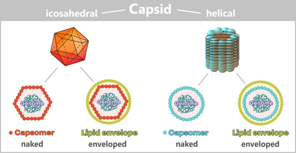
The capsid is the outer protein shell of a virus that protects its genetic material and determines its external shape. It is made up of many identical building blocks (capsomers) that assemble into symmetrical structures. The most common capsid shapes are icosahedral (20-faced) and helical (spiral-shaped).
Additional components, such as a lipid envelope – derived from the host cell – can alter the external shape. As a result, many enveloped viruses appear „spherical”, even though the underlying capsid is usually icosahedral. In some cases, such as with bacteriophages, the structure deviates significantly: this is referred to as a complex morphology, often featuring an icosahedral head and a helical tail. These morphological differences form the basis for the structural classification of viruses.
Viral hallmark genes – signatures beyond the cellular world
The genes that code for capsid proteins are among the so-called hallmark genes. They are:
- highly conserved within the viral world,
- functionally essential for the viral life cycle,
- and not found in cellular organisms.
Many of these proteins share a very distinctive shape: the jelly-roll fold. This three-dimensional structure resembles a rolled sponge cake and gives the capsid protein remarkable stability. It is found in a wide range of viruses – from those that infect humans to viruses that exist only in ancient deep-sea microbes. Its striking architecture is so characteristic that researchers can identify even novel viruses based solely on this genetic signature.
Anyone who has seen it once will recognise it – like a symbol woven through the depths of evolution – an evolutionary signature, legible to anyone willing to look closely.
As shown, for example, by the work of Koonin et al: Despite all their diversity, viruses have a common, ancient genetic core – as if they were carrying the coat of arms of their ancestors.
Conclusion: Virus-specific genome segments are a unique defining feature!
Viruses defy simple definitions. They are neither classic living organisms nor mere clusters of molecules. But they carry a set of characteristics that makes them distinguishable – in their form, in their function, and in their history.
If something has been leaving its own genetic trace for billions of years – then it is real. Even if it doesn’t lead an independent life. Even if we cannot see it.
Questions & Answers
🟡 „Are viruses just exosomes with a PR department?”
No. Exosomes are biological packaging waste. Viruses come with their own blueprint – and a transport container with perfect geometry.
Anyone who confuses exosomes with viruses is also confusing Tupperware with spaceships.
🔬 „But we’ve never really seen them!”
Yes, we have. Electron microscopes provide images, and cryo-tomography even produces 3D videos at nanometer resolution.
Invisible? Only when the power’s off.
🧬 „Isn’t the RNA just random cellular debris?”
No. Viral RNA/DNA is unique, functional, and precisely organized – and reproducible across the globe.
Random? Then a clockwork would just be some metal – with team spirit and a good mood.
📦 „That capsid – couldn’t it just form on its own?”
Hardly. These nanoboxes with perfect symmetry are found only in viruses.
A soccer ball doesn’t just randomly form in the grass, either.
🌍 „Maybe it’s all just a measurement artifact?”
Then it’s an astonishingly global one. All laboratories detect the same sequences, structures, and properties.
Viruses don’t recognize lab boundaries – only reproducibility.
In the end, one truth remains:
Viruses are not fiction, not artifacts, not products of chance.
They are biology’s most precisely mapped source of unease –
real, reproducible, and everywhere.
Anyone who calls them cellular junk might as well believe
a Tesla is just an especially ambitious shopping cart.
Sources and links documenting the isolation and sequencing of viruses:
National Center for Biotechnology Information (NCBI) Virus Database:
NCBI Virus Database
The NCBI hosts a comprehensive database of viral genomes that have been sequenced by scientists around the world. Here, you can access thousands of viral genomes that have been isolated and sequenced.
GISAID (Global Initiative on Sharing Avian Influenza Data):
GISAID
GISAID is a platform primarily used for the sharing of sequence data on influenza and SARS-CoV-2 viruses. It provides detailed information on the sequencing and origin of these viruses.
European Nucleotide Archive (ENA):
ENA Browser
The ENA provides access to sequence data from viruses that have been isolated in laboratories around the world. This database is maintained by the European Bioinformatics Institute (EBI) and contains extensive information on viral genomes.
PubMed – Scientific articles on virus isolation and sequencing:
Example search query: „Virus Isolation and Sequencing“
PubMed is a search engine for scientific literature. You can use it to find specific studies on the isolation and sequencing of viruses.
6. Where Do Viruses Come From?
These questions push the boundaries of our knowledge. They touch not only on the origins of viruses but on the very foundations of life itself. Before we explore possible scenarios for their emergence, it’s worth stepping back to look at the bigger picture: the „Tree of Life” – as modern evolutionary research depicts it today.
6.1. The Tree of Life
All known forms of life – from bacteria to blue whales – share a common origin: LUCA, the Last Universal Common Ancestor. LUCA was not the first organism ever to exist, but the last common ancestor of all cellular life alive today – bacteria, archaea, and eukaryotes. An evolutionary crossroads, not a starting point.
What do we know about LUCA? He likely lived around 3.5 to 4 billion years ago, in a warm and still-young Earth. LUCA was cellular, already equipped with DNA, RNA, and proteins, and capable of converting energy – but still far from the complexity of modern cells. A prototype of life, from which everything else branched out.
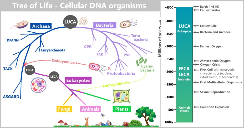
LUCA (Last Universal Common Ancestor) branches into the domains of Bacteria (e.g., Terrabacteria, Proteobacteria) and Archaea (e.g., Euryarchaeota, Asgard). Through the endosymbiotic fusion of a proteobacterium with an Asgard archaeon, FECA (First Eukaryotic Common Ancestor) emerges, which evolves into LECA (Last Eukaryotic Common Ancestor), the origin point for eukaryotes (animals, plants, fungi). A second endosymbiosis involving cyanobacteria gives rise to chloroplasts in plants. On the right, a timeline illustrates the emergence of life: from the formation of Earth (~4.5 billion years ago), through the Great Oxygenation Event (~2.4 billion years ago), to the Cambrian Explosion (~540 million years ago).
But while the Tree of Life grew full of branches, twigs, and leaves, one question remains unanswered: Where do viruses fit into this picture – or do they even belong on the tree at all?
Unlike bacteria or eukaryotes, viruses have no cellular structure, no metabolism of their own, and leave behind no fossils. Some scientists see them as „lost branches” of the Tree of Life, while others consider them ancient precursors – perhaps even predating LUCA itself.
To answer this question, we need to go back to the beginning – or rather, to the possible beginnings.
So where do viruses stand in this tree of life?
Are they late arrivals, evolved from derailed genes of cellular organisms? Or do they belong to the primordial forms of life – perhaps even older than LUCA itself?
Science has (as yet) no definitive answer. But several hypotheses aim to trace the origins of viruses.
6.2. The Main Hypotheses on the Origin of Viruses
💡Note: The following origin hypotheses assume a basic understanding of the so-called RNA world – an early phase in Earth’s history when life still consisted of simple, self-replicating RNA molecules. To immerse yourself in this unfamiliar era and better contextualize the hypotheses, we recommend the article „The First Whisper of Life”. It poetically tells the story of the beginnings of biological order – long before cells, proteins, and DNA.
6.2.1. Hypotheses in a Cellular World
These hypotheses assume the existence of cells from which viruses emerge.
6.2.1.a) Progressive Hypothesis – Viruses as Escaped Genes
6.2.1.b) Regressive Hypothesis – Viruses as Reduced Cellular Organisms

6.2.2. Hypotheses in the Pre-Cellular RNA World
These hypotheses place the origin of virus-like structures in a time before or during the formation of the first cells, in the RNA world, where self-replicating molecules dominated.
6.2.2.a) Virus-First Hypothesis – Viruses Came First
6.2.2.b) Co-Evolution Hypothesis – Viruses and Cells Emerged Together

6.2.1. Hypotheses in a Cellular World
The so-called Cell-First Hypothesis assumes that cellular life forms – such as LUCA – already existed before viruses emerged. Within this approach, two main scenarios can be distinguished:
a) The Progressive Hypothesis: According to this, viruses originate from genetic material that „escaped” from cells – essentially runaway genes that became independent and embarked on their own evolutionary path.
b) The Regressive Hypothesis: According to this idea, viruses were originally complete cells that have gradually reduced themselves over the course of evolution – until only the essential functions necessary for parasitic life remained. A kind of evolutionary reduction.
Both variants share a common idea: viruses are not an independent origin of life, but rather an evolutionary byproduct of cellular organisms – arising through loss or separation.
a) Progressive Hypothesis – Viruses as Escaped Genes
The Progressive Hypothesis – also known as the Escape Hypothesis – suggests that viruses originated from genetic material that was once part of cellular organisms. These „escaped genes” evolved over time into independent, infectious entities – detached from their original cellular context.
How could this have happened?
In living cells, there are small, mobile pieces of DNA or RNA that can move freely within the genome – so-called „jumping genes”. These elements, which include plasmids (circular DNA molecules) and transposons (DNA segments that can change their position within the genome), have the ability to replicate independently and even transfer between organisms.
The hypothesis states that some of these genetic elements evolved to the point where they eventually became capable of replicating independently. They escaped cellular control, developed protective mechanisms such as a capsid – a protein coat that shields their genetic material – and thus became the first viruses.
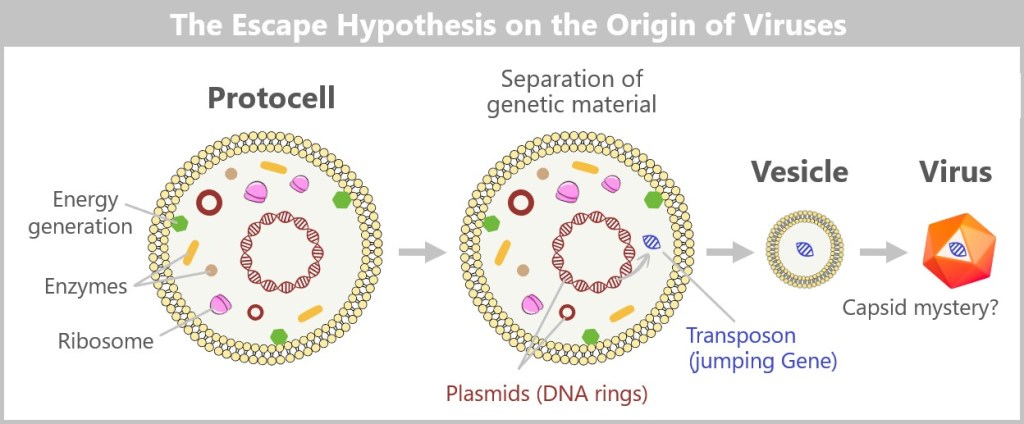
according to which viruses originated from originally cellular genes that gradually became independent.
Protocell: An early, simple cell form with genetic material: large DNA ring, ribosomes and smaller DNA rings.
Separation of genetic material: Mobile genetic elements – such as plasmids or so-called transposons („jumping genes”) – detach from the cell. These may have taken the first steps toward independence.
Vesicle formation: The separated genetic material is enclosed in small membrane-bound sacs (vesicles), providing protection and mobility.
Formation of a virus: Over the course of evolution, these developed into functional viruses – with a protective protein coat (capsid, orange). Exactly how this coat evolved remains unclear („capsid mystery?”).
✅ Arguments in Favor of This Hypothesis
➤ Similarity to Mobile Genetic Elements: Some viral genes closely resemble the „jumping genes” found within cells. Retroviruses in particular – such as HIV – use a mechanism similar to that of transposons: they reverse-transcribe their RNA into DNA and integrate it into the host’s genome.
➤ Viruses Exchange Genes with Their Hosts: Researchers have discovered genes in viral genomes that clearly originate from cellular organisms. This suggests that viruses may have once emerged from cells and, over time, acquired and evolved genetic material.
➤ Explanation for the Diversity of Viruses: Since different „jumping genes” may have escaped from different types of cells, this hypothesis helps explain why there are so many different viruses with varying characteristics.
❌ Weaknesses of the Hypothesis
➤ Capsid Proteins Are Extremely Ancient: Some key proteins involved in forming the viral shell (capsid) show no direct relation to cellular proteins. It remains unclear how escaped genes could have developed such complex structures. The evolution of these core proteins dates so far back that they may have existed even before the emergence of the first cellular life forms. A study by Krupovic & Koonin (2017) suggests that capsid genes may have evolved independently, before modern cells existed.
➤ Viruses Have Unique Enzymes That May Be Older Than LUCA: Some viruses contain RNA polymerases that differ significantly from those found in cells. These enzymes are so distinct that they may originate from a time before modern cellular mechanisms existed. Some researchers therefore speculate that viruses could be direct remnants of the RNA world – a phase of early evolution when life was still based on RNA rather than DNA.
➤ Viruses Exist in All Three Domains of Life: Viruses are found everywhere – they infect bacteria, archaea, and eukaryotes. If they had only emerged after the first cells evolved, one would expect them to be more confined to specific cellular lineages. Their universal presence suggests that they may have already existed before the split between bacteria, archaea, and eukaryotes.
➤ Viruses Do Not Share a Common Ancestry with Cellular Life: While bacteria, archaea, and eukaryotes can all be traced back to LUCA, there is no known common lineage for viruses. This suggests that viruses are not merely an offshoot of the cellular tree of life, but rather represent a very ancient, parallel line of evolution.
⬇️ Conclusion
The Cell-First Hypothesis views viruses as rebels of cellular life – originally harmless genetic passengers that broke away and followed their own evolutionary path. However, it assumes that complex cells already existed before viruses emerged.
b) Regressive Hypothesis – Viruses as Reduced Cellular Organisms
The Regressive or Reduction Hypothesis does not view viruses as fragments of escaped genes, but rather as former cells that gradually became more and more reduced over the course of evolution – until they lost their independence and turned into „gene packages” that rely on other cells to survive.
How could this have happened?
An early, complex, cellular organism (e.g., a parasite) developed an increasingly close dependence on its host. Over time, it lost unnecessary genes – for metabolism, cell division, and membrane formation – until it could no longer live independently. In the end, only a tiny remnant remained: the genes needed for replication (DNA/RNA), packaged in a protective shell (capsid) – a virus.

From a Traveling Cell Parasite to an Ultralight Virus
A free-living parasite (e.g., a small bacterium) infects another cell – just like some bacteria today parasitize other cells (e.g., Rickettsia or Chlamydia). Why? Probably because the protocell offered a safe environment. Perhaps the host had access to resources that the parasite couldn’t easily obtain – such as energy, enzymes, or nucleotides – a kind of molecular all-inclusive resort.
It is even possible that everything began symbiotically – similar to the mitochondria. It was only later that this relationship was exploited unilaterally – it became parasitic.
The parasite initially lived independently. It could leave the host cell or reproduce within it. But gradually, it needed fewer and fewer of its own genes – the host ultimately provided everything it required. So, the parasite gradually shed its genetic „baggage”, step by step.
Over time, through mutations or selection, it lost many of its original genes:
➤ It no longer produced its own proteins.
➤ It lost the ability to generate energy.
➤ Eventually, even the genes for cell division.
In the end, only its genome remained – packaged in a clever „case”: the capsid.
This is exactly where the virus comes into being: no longer an independent living organism in the classical sense, but an ultralight „traveler” that can only reproduce with the help of a host.
✅ Arguments in Favor of This Hypothesis
➤ Parallels to Intracellular Parasites: Some modern microorganisms, such as Rickettsia or Chlamydia, can only reproduce inside other cells – just like viruses. Moreover, their genomes are highly reduced. This demonstrates that cells can indeed undergo drastic „streamlining” through parasitism.
➤ Large DNA Viruses as „Transitional Forms”: Some giant viruses (e.g., Mimivirus, Pandoravirus) have incredibly large genomes – larger than some bacteria – and contain genes typically found in true cells (e.g., DNA repair enzymes). These viruses appear to act as evolutionary intermediates between real cells and typical viruses.
➤ Loss Instead of Creation: Evolution is not only about „more”, but often also about „less”. Especially in parasitic contexts, organisms frequently lose functions – just as assumed here.
❌ Weaknesses of the Hypothesis
➤ Origin Remains Unclear: Although the hypothesis explains how a cell could become a virus, it says little about when and under what conditions this might have occurred.
➤ No Common Ancestry: The diversity of viruses argues against a single „original cell” ancestor for all viruses. If all viruses descended from regressive cells, they would still have had to evolve independently multiple times. Some researchers therefore believe that regressive evolution is just one of several origins.
➤ Applies Mainly to Large DNA Viruses: This hypothesis fits well with large DNA viruses but less so with very simple RNA viruses, which lack any cell-like structures or genes.
➤ Capsid Proteins Show No Direct Similarity: Cells – even highly reduced parasitic ones – do not have capsids. The capsid is a virus-specific structure. If a virus evolved through reduction from a cell, the question arises: how could a structure like the capsid develop, which does not exist in cells at all? It appears to have arisen anew – which is difficult to reconcile with a theory based solely on „loss” and „reduction”.
➤ Energy Gap: Even degenerated parasites (e.g., Mycoplasma) retain metabolic genes – viruses have none.
⬇️ Conclusion
The Regressive Hypothesis views viruses not as „escaped gene fragments”, but as miniature versions of former cells. This idea is especially plausible for large DNA viruses: they may once have been fully functional cellular parasites that lost their independence through adaptation. In a way, they represent the biological opposite of evolution toward complexity – a regression to the core of survival: replication. However, the hypothesis falls short when explaining the diversity of simpler viruses.

6.2.2. Hypotheses in the Pre-Cellular RNA World
In the primordial soup of early Earth, something like life first began to stir – delicate, fleeting, yet profoundly significant. Molecules emerged that not only existed but acted: cutting, joining, and copying themselves. Inside tiny lipid bubbles that formed and disappeared, a network of cooperating and competing ribozymes grew (more on this in „The First Whisper of Life”).
It was not life in the modern sense. It was a game of possibilities. From this network, two evolutionary lines emerged:
① The stable, structure-loving replicators that became the first cells.
② And the free, reduced replicators that could be considered proto-viruses – mobile, adaptable, parasitic.
Early parasitism was less infection and more interaction – a dance between mutual benefit and exploitation rather than a true host invasion. Two hypotheses describe this origin:
a) Virus-First Hypothesis – Viruses Came First
b) Co-Evolution Hypothesis – Viruses and Cells Emerged Together
a) Virus-First Hypothesis – Viruses Came First
Which came first – the host or the virus?
The Virus-First Hypothesis gives a surprising answer: „Neither!” It postulates that virus-like replicators already existed in the RNA world – long before cells, DNA, or LUCA – as precursors of life.
The RNA World as an Incubator for Proto-Viruses
In this era, ribozymes (RNA molecules with enzymatic functions) were the first „survival artists”. Some became molecular parasites:
- They used other RNA strands as templates for copying („parasitism light”).
- They enclosed themselves in lipid vesicles or peptide rings (not yet true capsids).
- They replicated without cells – e.g., on clay minerals that acted as catalysts.
The leap to the modern virus: It was only with the emergence of cells that these replicators became efficient parasites – now able to hijack cellular machinery.

This graphic illustrates a possible evolutionary transition from prebiotic chemistry to the emergence of the first virus-like structures:
RNA World (left): Simple RNA molecules exist, some protected within lipid vesicles, with the ability to self-replicate.
Proto-Viruses (center): In this phase, the first parasitic RNA molecules (red) emerge. They can no longer replicate on their own but exploit other RNA strands (blue) instead. Encased in lipids and early peptides (short chains of amino acids), a primitive form of molecular parasitism begins. The red structures symbolize parasitic interactions between RNA molecules.
Cellular World (right): With the emergence of the first proto-cells, these strategies shift: RNA parasites (proto-viruses) leave their peptide vesicles and begin to infect cellular organisms – a primordial precursor of modern viruses.
✅ Arguments in Favor of This Hypothesis
➤ Unique viral enzymes: RNA polymerases found in viruses (such as in the influenza virus) show no resemblance to cellular proteins. This suggests a very ancient origin – possibly dating back to the RNA world, before the domains of life diverged.
➤ Unique capsid proteins: The protective shells viruses use to encase their genomes have no direct counterparts in cellular organisms – suggesting an early, independent evolutionary origin.
➤ Global distribution: Viruses infect all three domains of life – Bacteria, Archaea, and Eukarya. This suggests they originated before these domains diverged.
➤ Enormous diversity: The wide variety of viral genomes – RNA or DNA, single- or double-stranded – points to a long evolutionary history, possibly reaching back to the RNA world.
➤ Parallels to the RNA world: Many modern viruses carry RNA genomes. This aligns with the assumption that RNA was the original genetic material – and that viruses could be living relics of that time.
❌ Weaknesses of the Hypothesis
➤ Host dependency: Modern viruses rely on cellular machinery (e.g., ribosomes). How could they have replicated in the primordial soup without cells? Perhaps they used loose networks of self-replicating RNA molecules as „hosts”?
➤ Origin of capsids: The evolution of complex capsid structures remains unclear. Genuine capsid proteins require ribosomes – which did not yet exist. Proto-envelopes made of self-organizing peptides (e.g., short amino acid chains) or lipids might have stabilized RNA. The first capsid precursors could have developed in response to external stress or to better protect RNA – not as a parasitic mechanism, but as a survival advantage. However, the details remain speculative.
➤ No direct evidence: Viruses leave no fossils. Molecular traces from the RNA world have also not yet been detected – posing a general challenge in researching early life forms.
⬇️ Conclusion
The virus-first hypothesis is one of the most fascinating – and controversial – theories about the origin of life. It suggests that viruses were not latecomers but pioneers of evolution: molecular messengers that spread genetic information long before cells existed. They may even have been a catalyst for the emergence of more complex life. What began as molecular scramble eventually became the blueprint for modern viruses.
b) Co-Evolution Hypothesis – Viruses and Cells Emerged Together
Not cells first. Not viruses first.
But both together – in the dance of early evolution.
The co-evolution hypothesis assumes that viruses and cellular precursors developed in parallel – emerging from the same molecular primordial soup of the RNA world. It wasn’t an „either-or” scenario, but a dynamic interplay: replicators that challenged, exploited, and stabilized each other – thus laying the foundation for life.
The primordial soup as a testing ground
In early lipid vesicles – small, imperfect bubbles made of fats – RNA strands gathered. Some of these molecules replicated themselves, others helped with copying, and still others cut or joined sequences. Cooperation and competition began simultaneously.
Some replicators evolved into increasingly complex systems, from which the first proto-cells emerged. Others remained reduced, preferring to exploit existing structures rather than building their own – a kind of minimalist lifestyle reminiscent of early viruses.
An interplay emerges
In this scenario, parasitism wasn’t a later development but an original feature of molecular evolution.
- Viral precursors could influence proto-cells, for example through gene exchange or interference.
- Proto-cells, in turn, could stabilize or integrate virus-like replicators – for instance, as mobile genes or regulatory elements.
Thus, viruses and cells may have emerged from the same networks where everything was still fluid: independence, dependence, replication, competition.
No origin – but a relationship
The co-evolution hypothesis is less about explaining the „first virus” and more about viewing a relationship as old as life itself. According to this view, viruses were not subsequent troublemakers, but part of the system from the very beginning – co-players in the story of life.

The graphic illustrates the core idea of the co-evolution hypothesis: Viruses and cellular life forms originated from a shared molecular prehistory – the RNA world. Within lipid vesicles, networks of ribozymes coexisted and competed, giving rise to two distinct replicator strategies: some evolved into the precursors of stable proto-cells, while others reduced themselves to essentials and exploited external replication mechanisms – the early proto-viruses.
Even before the emergence of true cells, a kind of „molecular parasitism” began to take shape – not in the classical sense, but as an undirected exploitation of replication processes. With the appearance of cellular life forms, these interactions intensified: early viruses were now able to transfer genetic material between cells (horizontal gene transfer) or enter into complex – sometimes even cooperative – relationships with them. The rise of LUCA was therefore not the end of this co-evolution, but its first major climax.
✅ Arguments in Favor of This Hypothesis
➤ Avoiding the chicken-and-egg problem: This hypothesis elegantly sidesteps the question of whether viruses or cells came first: both developed in parallel from the same molecular precursors.
➤ Adaptation to the dynamics of the RNA world: The RNA world was not a linear process, but a network of cooperation and competition. This hypothesis reflects that diversity more accurately than a model with a single, clear origin path.
➤ Explanation of viral diversity: Different virus groups (RNA, DNA, retroviral elements) could have evolved independently, but within the same molecular environment – which plausibly accounts for their tremendous diversity.
➤ Evolutionary interaction: Co-evolution explains why cell-like and virus-like systems interacted with each other from an early stage (e.g., through horizontal gene transfer, RNA competition, and mutual adaptation).
➤ Viruses as drivers of cellular complexity: Viruses might not have been just „parasites” but also catalysts of cellular evolution, for example through gene transfer, regulation, and the development of immune and defense mechanisms.
❌ Weaknesses of the Hypothesis
➤ Conceptual vagueness: At what point is a replicator considered a „virus” and when a „cell”? The transitions are fluid, which makes the hypothesis insightful but also difficult to clearly define or test.
➤ Lack of fossils: As with the virus-first hypothesis, there are no direct traces of early viral replicators. Molecular fossils from the RNA world simply do not exist.
➤ Complexity problem: Even in this hypothesis, it remains unclear where certain virus-specific proteins – such as capsid or polymerase proteins – originally came from. The formation of genuine capsids, efficient replication, and host exploitation requires complex proteins whose origins are still unknown – especially considering that ribosomes did not yet exist.
➤ Experimentally difficult to verify: The hypothesis is theoretically well-founded but hardly directly testable. Simulations and conclusions often remain speculative.
⬇️ Conclusion
The co-evolution hypothesis offers a flexible, systemic perspective on the early history of life – without committing to a linear cause-and-effect chain. It fits well with the chaotic and cooperative conditions of the RNA world. According to this model, viruses are not simply „descendants of cells” or „primordial ancestors”, but rather evolutionary contemporaries – equally ancient, equally significant, yet traveling a very different path.
Viruses are the hieroglyphs of biology
…we decipher them, but their origin remains a mystery.
Like flickering shadows on a cave wall:
- sometimes renegade parts of cells,
- sometimes runaway genes,
- sometimes the ancestors of life itself.
Maybe the question of their origin isn’t about the single source, but many evolutionary pathways – paths that intersect, overlap, and feedback into each other. The classic hypotheses (Virus-first, Co-Evolution, Progressive, Regressive) don’t have to contradict one another – they might have played out at different points in history.
And perhaps the question of origin isn’t the essential one at all. Viruses compel us to grasp something deeper:
Life is not a state, but a process – and viruses are its restless pulse.
They remind us that evolution is not a straight-lined tree, but a swirling river of cooperation, theft, and reinvention. Where did they come from? We don’t know. That they will remain? Certainly.
Perhaps that’s exactly why they fascinate us – because they show that life never stands still.
Further sources
The origins of viruses: evolutionary dynamics of the escape hypothesis
Viruses take center stage in cellular evolution
The origin of viruses and their possible roles in major evolutionary transitions
A virocentric perspective on the evolution of life
How did Viruses Evolve and How are They Related to Cellular Life?
Viruses and cells intertwined since the dawn of evolution
The origin of viruses and their possible roles in major evolutionary transitions
The ancient Virus World and evolution of cells
Virus-First Hypothesis • Viruses older than life?
What viruses tell us about evolution and immunity: beyond Darwin?
Were viruses around on Earth before living cells emerged? A microbiologist explains
7. Why Do Viruses Exist?
The short answer: Because there always has to be something that disrupts.
Sounds funny – but it’s a law of nature:
Nothing stays alive if it’s never challenged.
You can say many things about viruses.
That they aren’t alive.
That they only disrupt and destroy.
That they’re mere molecular parasites – dependent on the life they infect.
And yet: Without them, much would not be as it is.
Perhaps we wouldn’t even exist.
Life needs repetition. And deviation.
The story of life didn’t begin with a goal.
It began with repetition.
Again and again, molecules joined, broke apart, and rejoined.
Not because they had to – but because they could.
What repeats eventually becomes probable.
What works, stays.
What stays, must change.
And change needs deviation.
Mutation. Error. Disruption.
Without them, there would be no diversity, no evolution – no story.
Order is inertia. Life is movement.
When the first stable systems emerged, it was a triumph –
but also a risk.
Because what is stable tends toward rigidity.
What functions too perfectly dares nothing new.
But life needs movement.
This is where viruses begin to play their role –
not as enemies of life, but as a counterforce.
They challenge.
They disrupt.
They push cells into defense – and into innovation.
The duality: Order vs. Chaos
Cells build walls, viruses leap over them.
Their relationship is a paradoxical symbiosis:
They kill – and make life possible,
keep ecosystems running,
and even gave us placenta genes.
Viruses are not mistakes – they are a principle.
They are boundary violators, not out of malice, but out of principle.
They keep life permeable. Open. Vigilant.
They transfer genes, open up new paths, shake up systems.
Not always for the better.
But always with impact.
Maybe viruses are exactly what life needs to stay alive.
Not as an opposing model – but as a co-player, as the shadow cast by life itself.
The Tree of Life – permeated by viruses
When we look today at the Tree of Life, at its branches, twigs, and forks – we see the cells, the species, the visible trace of evolution.
And the viruses?
Missing.
Not because they are unimportant – but because they cannot be pinned down.
They are neither branch nor leaf, but the wind that moves them.
They are the whisper between the branches.
No distinct lineage, no part of the wood – and yet everywhere.
A stream of information that not only surrounds the tree but also shapes it.
They are the points between the lines, creating connections.
Waves of disruption that force growth.
Deviations that do not destroy the pattern but expand it.
They are the dark matter of biology: invisible, yet permeating everything.
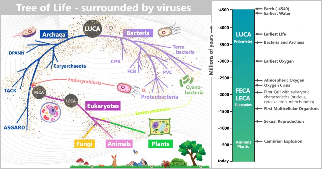
The „Tree of Life” illustrates the lineage of cellular organisms – Bacteria, Archaea, and Eukaryotes – tracing back to their last universal common ancestor (LUCA). The tiny dots and lines represent viruses: not as distinct branches, but as a diffuse network permeating the entire tree.
In this view, viruses are not outsiders but creative variants of molecular evolution. They are not entities with a clear lineage, but recurring phenomena in a universe that plays with variation and repetition.
And that is why they exist.
Not because they want to. Not because they have to.
But because they keep emerging – wherever nature varies.
Where life organizes itself – and from that order dares something new.
They exist because they are unavoidable.
Like an echo of the principle underlying everything:
Disruption is not the opposite of life.
Disruption is its possibility.
Viruses exist because disruption is not an accident –
but the universe’s tool to keep life awake and alive.
Remember this the next time a virus annoys you:
Maybe it’s just the universe giving you a cosmic slap –
and mumbling:
„Come on, wake up! Here’s your daily dose of chaos – so you can keep evolving.”
Epilogue: The Inconspicuous Ones
Viruses are the sand in the gears of creation.
Without will, without body –
and yet the invisible hand
that writes evolution.
The whisper between the lines of life –
not out of intent, but out of necessity.
They emerged from the mist of beginnings
and lingered in the shadows –
not as foreign bodies, but as an opponent,
as a touchstone and as an impulse.
They teach us humility:
For what destroys,
can also create.
Maybe that’s their message:
That life doesn’t grow against chaos,
but dances with it.
Addendum:
I approached this topic as a complete layperson. And that turned out to be an advantage – because I knew what I didn’t know.
With curiosity, skepticism, and a sense of wonder, I delved into the world of viruses – and was astonished by the unexpected dimensions that unfolded. This subject carries a weight of insight I never would have anticipated.
During my process of searching, questioning, and formulating, I had tremendous support from AI systems like ChatGPT and DeepSeek. The dialogue with these tools not only accelerated my learning but also deepened it. Without their assistance, I would have missed many things – and certainly wouldn’t have been able to articulate them so clearly.
What has emerged here is the result of human curiosity and machine patience. And it shows that learning today can be more than ever a collaborative process – one that crosses boundaries, even those between human and machine.
Sources (as of 07.07.2025)
